4.1: Activity 1 - Hash Tables

Introduction

To store a key/value pair we can use a simple array like data structure where keys directly can be used as index to store values. But in case when keys are large and can’t be directly used as index to store value, we can use a technique of hashing. In hashing, large keys are converted into small ones, by using hash functions and then the values are stored in data structures called hash tables.

The goal of hashing is to distribute the entries (key / value pairs) across an array uniformly. Each element is assigned a key (converted one) and using that key we can access the element in O(1) time. Given a key, the algorithm (hash function) computes an index that suggests where the entry can be found or inserted. Hashing is often implemented in two steps:

• The element is converted into an integer, using a hash function, and can be used as an index to store original element, which falls into the hash table.
• The element is stored in the hash table, where it can be quickly retrieved using a hashed key. That is,

hash = hashfunc(key)

index = hash % array_size

In this method, the hash is independent of the array size, and it is then reduced to an index (a number between 0 and array_size − 1), using modulo operator (%).

A hash table data structure attracts a wide use including:

• Associative arrays - Hash tables are commonly used to implement many types of in-memory tables. They are used to implement associative arrays (arrays whose indices are arbitrary strings or other complicated objects).
• Database indexing - Hash tables may also be used as disk-based data structures and database indices (such as in dbm).
• Caches - Hash tables can be used to implement caches, auxiliary data tables that are used to speed up the access to data that is primarily stored in slower media.
• Object representation - Several dynamic languages, such as Perl, Python, JavaScript, and Ruby, use hash tables to implement objects.

Hash functions are used in various algorithms to make their computing faster.

Activity Details

A hash function is any function that can be used to map dataset of arbitrary size to dataset of fixed size which falls into the hash table. The values returned by a hash function are called hash values, hash codes, hash sums, or simply hashes. In order to achieve a good hashing mechanism, it is essential to have a good hash function. A good hash function has three basic characteristics:

1. Easy to compute – A hash function should be easy to compute. It should not become an algorithm in itself.

2. Uniform distribution – It should provide a uniform distribution across the hash table and should not result in clustering.

3. Less collisions – Collision occurs when pairs of elements are mapped to the same hash value. It should avoid collisions as far as possible.

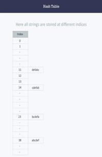
Note that no matter how good a hash function may be, collisions are bound to occur. So, they need to be managed through various collision resolution techniques in order to maintain high performance of the hash table. To understand the need for good hash functions consider the following example: Suppose it is required to store strings in the hash table using hashing {“abcdef”, “bcdefa”, “cdefab” , “defabc” }. To compute the index for storing the strings, the hash function that states “the index for a particular string will be equal to the sum of the ascii values of the characters modulo 599” should be used. As 599 is prime number, it will reduce the possibility of same index for different strings (collisions). It is thus recommended to use prime number when using modulo.

As we know ascii value of a = 97, b = 98, c= 99, d = 100, e = 101, f = 102. As all the strings contain same characters with different permutations, so the sum for each will be the same, that is, 599. So the hash function will compute same index for all the strings, and strings will be stored in the hash table in the format given in Figure 4.1.1 . As the index of all the strings is same, so we can create a list on that particular index and can insert all the strings in that list. So to access a particular string, it will take O(n) time where n is the number of strings, which shows that the hash function is not a good hash function.

Figure 4.1.1 : A hash table with strings on same index

Table 4.1.1 : String-index mapping for updated hash function

String	Hash function	Index
abcdef	(971 + 982 + 993 + 1004 + 1015 + 1026)%2069	38
Bcdefa	(981 + 992 + 1003 + 1014 + 1025 + 976)%2069	23
Cdefab	(991 + 1002 + 1013 + 1024 + 975 + 986)%2069	14
Defabc	(1001 + 1012 + 1023 + 974 + 985 + 996)%2069	11

Figure 4.1.2 : A hash table resulting from updated hash function

A hash table is a data structure used to store key / value pairs. Hash tables use a hash function to compute an index into an array where the element will be inserted or searched. By using a good hash function, hashing can perform extremely well. Under reasonable assumptions, the average time to search for an element in a hash table is O(1).

Consider a string S defined below:

string S = “ababcd”

Suppose we need to count the frequency of all the characters in the string S. The simplest thing to do would be to iterate over all the possible characters and count their frequency one by one. The time complexity of this approach is O(26*N) where N is the size of the string and there are 26 possible characters (in English alphabet). The function defined below performs this task.

void countFre(string S)
{ for(char c = ‘a’;c <= ‘z’;++c)
    {   int frequency = 0;
        for(int i = 0;i < S.length();++i)
            if(S[i] == c)
                frequency++;
cout << c << ‘ ‘ << frequency << endl; }

The output of the function above for input S is: a(2), b(2), c(1), d(1), e(0), f(0), …, z(0), where the number in brackets denotes the frequency.

To apply hashing to this problem, we define an array ‘Frequency’ of size 26 and hash the 26 characters with indices of the array using the hash function. Subsequently, iterate over the string and for each character, and increase the value in ‘Frequency’ at the corresponding index. The complexity of this approach is O(N) where N is the size of the string. Below we define a function that uses this method.

int Frequency[26];
int hashFunc(char c)
{   return (c - ‘a’);    }
void countFre(string S)
{   for(int i = 0;i < S.length();++i)
    {   int index = hashFunc(S[i]);
        Frequency[index]++;    }
    for(int i = 0;i < 26;++i)
        cout << (char)(i+’a’) << ‘ ‘ << Frequency[i] << endl;}

The output of this function for the input S is a(2), b(2), c(1), d(1), e(0), f(0), …, z(0), where the number in brackets denotes frequency.

We define a load factor as the number of entries divided by the size of the hash table, i.e., n / k where n is the number of entries and k is the size of the hash table. If the load factor is kept reasonable, the hash table will perform well, if the hash function used is good. If the load factor grows too large, the hash table will become slow, or it may fail to work (depending on the hash function used). The expected constant time property of a hash table assumes that the load factor is kept below some bound. A low load factor is not especially beneficial, since as the load factor approaches 0, the proportion of unused areas in the hash table increases. This will result in wasted memory.

Collision Resolution Techniques

Separate chaining (Open hashing) - Separate chaining is one of the most common and widely used collision resolution techniques. It is usually implemented using linked lists. In separate chaining, each element of the hash table is a linked list. To store an element in the hash table, simply insert into a particular linked list. If there is any collision, i.e., two different elements have same hash value, then store both elements in the same linked list. Figure 4.1.3 depicts a hash table with separate chaining resolution.

Figure 4.1.3 : Separate chaining

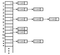
The cost of a lookup is that of scanning the entries of the selected linked list for the desired key. If the distribution of keys is sufficiently uniform, the average cost of a lookup depends only on the average number of keys per linked list, i.e., it is roughly proportional to the load factor. For this reason, chained hash tables remain effective even when the number of table entries n is much higher than the number of slots.

For separate-chaining, the worst-case scenario is when all entries are inserted into the same linked list. The lookup procedure may have to scan all its entries, so the worst-case cost is proportional to the number n of entries in the table.

Figure 4.1.4 : Hash table with separate chaining

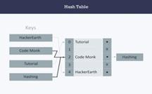
In Figure 4.1.4 , the keys Code Monk and Hashing both hash to the value 2. But, the linked list at index 2 can hold only one entry, thus the next entry, in this case Hashing is linked (attached) to the entry of Code Monk. The implementation of hash table with separate chaining is presented below with an assumption that the hash function will return an integer from 0 to 19.

vector <string> hashTable[20];
int hashTableSize=20;
//insertion
void insert(string s)
{            // Compute the index using Hash Function
    int index = hashFunc(s);
    // Insert the element in the linked list at the particular index
    hashTable[index].push_back(s); } 
//searching
void search(string s)
{   // Compute the index using Hash Function
    int index = hashFunc(s);
    // Search the linked list at that particular index 
    for(int i = 0;i < hashTable[index].size();i++)
    {    if(hashTable[index][i] == s)
        {    cout << s << “ is found!” << endl;
        return;    }
    cout << s << “ is not found!” << endl; }

Linear probing (Open addressing or Closed hashing) - In open addressing, all entry records are stored in the array itself, instead of linked lists. When a new entry need to be inserted, a hashed index of hash value is computed and the array is examined, starting with the hashed index. If the slot at hashed index is unoccupied, the entry record is inserted in slot at hashed index; otherwise, proceed with a probe sequence, until an unoccupied slot is found.

A probe sequence is the sequence followed while traversing through the entries. There may be different interval between successive entry slots or probes in different probe sequence. When searching for an entry, the array is scanned in the same sequence, until either the target element is found, or an unused slot is found, which indicates that there is no such key in the table. The name “open addressing” refers to the fact that the location (“address”) of the item is not determined by its hash value. Linear probing is when the interval between successive probes is fixed (usually to 1).

Suppose the hashed index for a particular entry is index. A probing sequence for linear probing is given by

index = index % hashTableSize

index = (index + 1) % hashTableSize

index = (index + 2) % hashTableSize

index = (index + 3) % hashTableSize

and so on…

Figure 4.1.5 : Hash table with linear probing

Figure 4.1.5 shows an example of hash collision resolved by open addressing with linear probing.

Note that since the keys Code Monk and Hashing are hashed to the same index, i.e., 2, thus the key Hashing is stored at index 3 as the interval between successive probes is 1. The implementation of hash table with linear probing is presented below with an assumption that there are no more than 20 elements in the data set and the hash function return an integer from 0 to 19, and that data set have unique elements.

string hashTable[21];
int hashTableSize = 21;
//insertion
void insert(string s)
{    // Compute the index using the Hash Function 
    int index = hashFunc(s);
    // Search for an unused slot and if the index will exceed the hashTableSize
    // we will roll back
    while(hashTable[index] != “”)
        index = (index + 1) % hashTableSize; 
    hashTable[index] = s; }
//searching
void search(string s)
{   // Compute the index using the Hash Function
    int index = hashFunc(s);
    // Search for an unused slot and if the index will exceed the hashTableSize
    // we will roll back
    while(hashTable[index] != s and hashTable[index] != “”)
        index = (index + 1) % hashTableSize;
    // Element is present in the Hash Table or not 
    if(hashTable[index] == s)
        cout << s << “ is found!” << endl;
    else
        cout << s << “ is not found!” << endl; }

Quadratic probing - Quadratic probing is same as linear probing, the only difference being the interval between successive probes or entry slots. When at hashed index for an entry record whose slot is already occupied, start traversing until there is no more unoccupied slot. The interval between slots is computed by adding the successive value of arbitrary polynomial in the original hashed index. Suppose that the hashed index for an entry is index, and the slot at index is occupied, the probe sequence proceeds as follows:

index = index % hashTableSize

index = (index + 12) % hashTableSize

index = (index + 22) % hashTableSize

index = (index + 32) % hashTableSize

and so on…

The implementation of hash table with quadratic probing is given below with assumptions that there are no more than 20 elements in the data set thus hash function will return an integer from 0 to 19, and the data set have unique elements.

string hashTable[21];
int hashTableSize = 21;
//insertion
void insert(string s)
{   // Compute the index using the Hash Function
    int index = hashFunc(s);
        // Search for an unused slot and if the index will
        // exceed the hashTableSize we will roll back 
    int h = 1;
    while(hashTable[index] != “”)
    {   index = (index + h*h) % hashTableSize;
        h++;    }
    hashTable[index] = s; }
//Searching
void search(string s)
{   // Compute the index using the Hash Function 
    int index = hashFunc(s);
    // Search for an unused slot and if the index will exceed the hashTableSize
    // we will roll back
    int h = 1;
    while(hashTable[index] != s and hashTable[index] != “”)
    {   index = (index + h*h) % hashTableSize;
        h++;    }
    // Element is present in the Hash Table or not 
    if(hashTable[index] == s)
        cout << s << “ is found!” << endl;
    else
        cout << s << “ is not found!” << endl; }

Double hashing - Double hashing is same as linear probing, the only difference being the interval between successive probes. The interval between probes is computed by using two hash functions. That is, suppose that the hashed index for an entry record is index which is computed by one hashing function and at index the slot is already occupied, then we start traversing in a particular probing sequence to look for unoccupied slot as shown below where indexH is the hash value computed by another hash function.

index = (index + 1 * indexH) % hashTableSize;

index = (index + 2 * indexH) % hashTableSize;

and so on….

The implementation of hash table with double hashing is given below with the assumptions that there are no more than 20 elements in the data set thus hash functions will return an integer from 0 to 19, and the data set have unique elements.

string hashTable[21];
int hashTableSize = 21;
//insertion
void insert(string s)
{   // Compute the index using the Hash Function1
    int index = hashFunc1(s);
    int indexH = hashFunc2(s);
    // Search for an unused slot and if the index will exceed the hashTableSize
    // we will roll back
    while(hashTable[index] != “”)
        index = (index + indexH) % hashTableSize;
    hashTable[index] = s; }
//searching
void search(string s)
{   // Compute the index using the Hash Function
    int index = hashFunc1(s);
    int indexH = hashFunc2(s);
    // Search for an unused slot and if the index will exceed the hashTableSize
    // we will roll back
    while(hashTable[index] != s and hashTable[index] != “”)
        index = (index + indexH) % hashTableSize;
    // Element is present in the Hash Table or not 
    if(hashTable[index] == s)
        cout << s << “ is found!” << endl;
    else
        cout << s << “ is not found!” << endl;}

Conclusion

This activity presented the hash table data structure. Hash tables use hash functions to generate indexes for keys to be stored or accessed from array/list. They find a wide use including implementation of associative arrays, database indexes, caches and object representation in programming languages. A good hash function design is instrumental to the hash table performance whose expected access time is O(1). Hash functions suffer from collision problems where two different keys get hashed/mapped to the same index. Collision can be addressed through use of collision resolution techniques, including separate chaining, linear probing, double hashing and quadratic probing.

Assessment

1. Given a hash table with m=11 entries and the hash function h1 and second hash function h2:

   h1(key) = key mod m

   h2(key) = {key mod (m-1)} + 1

   Insert the keys {22, 1, 13, 11, 24, 33, 18, 42, 31} in the given order, i.e., from left to right, to the hash table using each of the following hash methods:

   1. Separate Chaining
   2. Linear probing
   3. Double hashing

2. Suppose a hash table with capacity m=31 gets to be over ¾ full. We decide to rehash. What is a good size choice for the new table to reduce the load factor below 0.5 and also avoid collisions?