4.2: Activity 2 - Graphs

Introduction

Consider a social network such as facebook which is an enormous network of persons including you, your friends, family, their friends and their friends, etc. This is referred to as a social graph. In this graph, every person is considered as a node of the graph and the edges are the links between two people. In facebook, friendship is a bidirectional relationship. That is if A is B’s friend it implies also that B is A’s friend, thus the associated graph is an undirected graph.

A graph is defined as a collection of finite sets of vertices or nodes (V) and edges (E). Edges are represented as ordered pairs (u, v), where (u, v) indicates that there is an edge from vertex u to vertex v. Edges may contain cost, weight or length. The degree of a vertex is the number of edges that connect to it. A path is a sequence of vertices in which every consecutive vertex pair is connected by an edge and no vertex is repeated in the sequence except possibly the start vertex. There are two types of graphs:

Undirected graph - a graph in which all the edges are bidirectional, essentially the edges don’t point in a specific direction. Figure 4.2.1 depicts an undirected graph on four vertices and four edges.

Figure 4.2.1 : An undirected graph

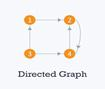
Directed graph (digraph) - a graph in which all the edges are unidirectional. Figure 4.2.2 depicts a digraph on four vertices and five directed edges (arcs).

Figure 4.2.2 : A directed graph

A weighted graph has each edge assigned with a weight or cost. Consider a graph of 4 nodes depicted in Figure 4.2.3 . Observe that each edge has a weight/cost assigned to it. Suppose we need to traverse from vertex 1 to vertex 3. There are 3 possible paths: 1 -> 2 -> 3, 1 -> 3 and 1 -> 4 -> 3. The total cost of path 1 -> 2 -> 3 is (1 + 2) = 3 units, the total cost of path 1 -> 3 is 1 units and the total cost of path 1 -> 4 -> 3 is (3 + 2) = 5 units.

Figure 4.2.3 : A weighted graph

A graph is called cyclic if there is a path in the graph which starts from a vertex and ends at the same vertex, and this path is called a cycle. An acyclic graph is a graph which has no cycle. A tree is an undirected graph in which any two vertices are connected by only one path. A tree is acyclic graph and has N - 1 edges where N is the number of vertices. Figure 4.2.4 shows a tree on 5 nodes.

Figure 4.2.4 : A tree

Activity Details

Graph Representation

There is variety of ways to represent a graph, but the two most popular approaches are the adjacency matrix and adjacency list. Adjacency matrix is a V x V binary matrix (i.e., a matrix in which the cells can have only one of two possible values, either a 0 or 1), where an element Ai,j is 1 if there is an edge from vertex i to vertex j else Ai,j is 0. The adjacency matrix can also be modified for the weighted graph in which instead of storing 0 or 1 in Ai,j, store the weight or cost of the edge from vertex i to vertex j. In an undirected graph, if Ai,j = 1 then Aj,i = 1. In a directed graph, if Ai,j = 1 then Aj,i may or may not be 1. Adjacency matrix provide a constant time access, that is, O(1) to check whether there is an edge between two nodes. The space complexity of adjacency matrix is O(V²). Figure 4.2.5 presents a graph and its adjacency matrix.

i/j: 1 2 3 4

1: 0 1 0 1

2: 1 0 1 0

3: 0 1 0 1

4: 1 0 1 0

Figure 4.2.5 : A four node graph and corresponding adjacency matrix

i/j: 1 2 3 4

1: 0 1 0 0

2: 0 0 0 1

3: 1 0 0 1

4: 0 1 0 0

Figure 4.2.6 : A digraph and corresponding adjacency matrix

Adjacency list represents a graph as an array of separate lists. Each element of the array Ai is a list which contains all the vertices that are adjacent to vertex i. For weighted graph we can store weight or cost of the edge along with the vertex in the list using pairs. In an undirected graph, if vertex j is in list Ai then vertex i will be in list Aj.

The space complexity of adjacency list is O(V + E) because in adjacency list we store information for only those edges that exist in the graph. Note that for cases where a matrix is sparse (i.e., most matrix elements entries, by contrast, if most entries are nonzero the matrix is considered dense), using an adjacency matrix might not be very useful, since a lot of space is used, though mostly occupied by 0 entries. In such cases an adjacency list would be a better choice. Figure 4.2.7 presents an undirected graph along with it adjacency list. Similarly, Figure 4.2.8 presents a digraph with its corresponding adjacency list.

A1→2→4

A2→1→3

A3→2→4

A4→1→3

Figure 4.2.7 : A graph and its adjacency list

A1→2

A2→4

A3→1→4

A4→2

Figure 4.2.8 : A digraph along with its adjacency list

Graph Traversals

Some graph algorithms may require that every vertex of a graph be visited exactly once. The order in which the vertices are visited may be important, and may depend upon a particular algorithm or particular question being solved. During a traversal, we may keep track of which vertices have been visited so far. The most common way is to mark the vertices which have been visited. A graph traversal visits every vertex and every edge exactly once in some well-defined order. There are many approaches to traverse a graph. Two most popular traversal methods are the depth first search (DFS) and breadth first search (BFS).

The DFS traversal is a recursive algorithm that uses the idea of backtracking. Basically, it involves exhaustive searching of all the nodes by going ahead whenever possible, otherwise it backtracks. Backtracking means that when cannot get any further node in the current path, move back to the node from where can find further nodes to traverse. That is, continue visiting nodes as long as unvisited nodes are found along the current path, when current path is completely traversed select a next path.

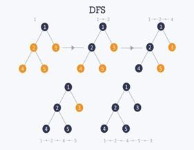
The recursive nature of DFS can be implemented using stacks. The basic idea is, pick a starting node and push all its adjacent nodes into a stack. Pop a node from stack to select the next node to visit and push all its adjacent nodes into a stack. Keep on repeating this process until the stack is empty. DFS do not visit a node more than once, otherwise, might end up in an infinite loop. To avoid an infinite loop, DFS marks the nodes as soon as they are visited. The pseudo-code for DFS is presented below both for an iterative and recursive version. Figure 4.2.9 illustrates the DFS steps on a five node tree.

DFS-iterative (G, s):     //where G is graph and s is source vertex.
    let S be stack
    S.push( s )     // inserting s in stack mark s as visited.
    while ( S is not empty):
        // pop a vertex from stack to visit next
        v = S.top( )
        S.pop( )
        //push all the neighbours of v in stack that are not visited
        for all neighbours w of v in Graph G:
            if w is not visited :
                S.push( w )
                mark w as visited
DFS-recursive(G, s):
    mark s as visited
    for all neighbours w of s in Graph G:
        if w is not visited:     DFS-recursive(G, w)

Figure 4.2.9 : A DFS traversal on a tree

A BFS traversal starts from a selected node (source or starting node) and proceeds to traverse the graph layer-wise, that is, explores the neighboring nodes (nodes which are directly connected to source node) and subsequently proceed towards the next level neighbor nodes. Therefore BFS move in breadth of the graph, that is, moves horizontally first and visit all the nodes of the current layer and then to the next layer. Figure 4.2.10 illustrates a BFS traversal.

Figure 4.2.10 : A BFS traversal

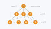
Note from Figure 4.2.10 that a BFS traversal, visits all nodes on layer 1 before proceeding to nodes of layer 2, since nodes on layer 1 have less distance from source node compared to nodes on layer 2. Since a graph may contain cycles, BFS may possibly visit the same node more than once when traversing the graph. To avoid processing a node more than once, a boolean array may be used to track already processed nodes. While visiting the nodes of current layer of graph, they are stored such that the child nodes are also visited in the same order as the respective parent node.

In Figure 4.2.10 the BFS starts from 0, visit its children 1, 2, and 3 and store them in the order they get visited. Upon visiting all vertices of current layer, BFS proceeds to visit the children of 1 (i.e., 4 and 5), 2 (i.e., 6 and 7) and 3 (i.e., 7) in that order, and so on.

To simply the implementation of the above process, use a queue to store the node and mark it as visited, and should remain in queue until all its neighbors (vertices which are directly connected to it) are marked as visited. Since a queue follows FIFO order (First In First Out), BFS will first visit the neighbors of that node, which were inserted first in the queue. Below a pseudo code for BFS is presented, and Figure 4.2.11 shows a BFS traversal on a six node graph.

//BSF Pseudocode
BFS (G, s)     //where G is graph and s is source node.
    let Q be queue.
    Q.enqueue( s ) // inserting s in queue until all its neighbour vertices are marked.
    mark s as visited.
    while ( Q is not empty)
        // removing that vertex from queue, whose neighbour will be visited now.
        v = Q.dequeue( )
        //processing all the neighbours of v
        for all neighbours w of v in Graph G
            if w is not visited
                Q.enqueue( w )     //stores w in Q to further visit its neighbour
                mark w as visited.

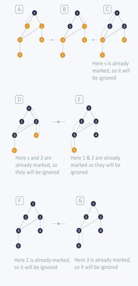
The BFS traversal on Figure 4.2.11 proceeds as follows: Starting from source node s push in queue and mark it visited. In first iteration, pops s from queue and traverse on neighbors of s, that is 1 and 2. Since 1 and 2 are unvisited, they are pushed in queue and be marked as visited.

In second iteration, pops 1 from queue and traverse its neighbors s and 3. Since s is already marked visited, it is ignored and 3 is pushed in queue and marked as visited.

In third iteration, pops 2 from queue and traverse its neighbors s, 3 and 4. Since 3 and s are already marked visited, they are ignored and 4 is pushed in queue and marked as visited. In fourth iteration, pops 3 from queue and traverse its neighbors 1, 2 and 5. Since 1 and 2 are already marked visited, they are ignored and 5 is pushed in queue and marked as visited.

In fifth iteration, pops 4 from queue and traverse its neighbor, that is, 2. Since 2 is already marked visited it is ignored. In sixth iteration, pops 5 from queue and traverse its neighbors, that is, 3. Since 3 is already marked visited it is ignored. Eventually, the queue is empty so it comes out of the loop. Through this process all the nodes have been traversed by BFS.

Figure 4.2.11 : A BFS traversal

The time complexity of BFS is O(V + E), where V is the number of nodes and E is the number of Edges.

Conclusion

This activity presented the graph data structure which is defined by a set of vertices and edges. Graph data structure is very useful in problems which can be modelled as a network. Two graph representation techniques were presented, the adjacency matrix and adjacency list approach. When processing a graph a systematic visitation of its nodes can be facilitated by DFS and BFS traversals.

Assessment

1. Consider a weighted graph in Figure 4.2.12 , with A being a start vertex.

   

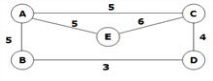
   Figure 4.2.12

   1. Define its adjacency matrix
   2. Define its adjacency list
   3. List the vertices using DFS
   4. List the vertices using BFS