4.3: Activity 3 - Graph Algorithms

Introduction

In this activity we will explore two graph algorithms, the topological sort and shortest path algorithms. The topological sort algorithm takes as input a directed acyclic graph and generates a linear sequence of vertices that are totally order by vertex precedence. This algorithm finds wide applications including in projects planning and scheduling, detection of cycles and in creation of software builds with module dependency.

The shortest path problem seeks to find a path between two vertices in a graph such that the sum of the weights of its constituent edges is minimized. We consider the Dijkstra algorithm that finds the shortest path for a single source graph with non-negative edge weights, and the Bellman Ford algorithm which works even for graphs with negative edge weights. Furthermore, we consider the Floyd-Warshall algorithm which finds shortest paths in multiple sourced graph setting with arbitrary edge weights. Shortest path algorithms have wide range of applications, both direct and as a sub-problem of other problems. Some of the prominent applications include in vehicle routing and network design and routing.

Activity Details

Topological Sort

A cycle in a digraph G is a set of edges, {(v1, v2), (v2, v3), ..., (vr −1, vr)} where v1 = vr. A digraph is acyclic if it has no cycles. Such a graph is often referred to as a directed acyclic graph, or DAG, for short. DAGs are used in many applications to indicate precedence among events. For example, applications of DAGs include depict/model the following:

• inheritance in object oriented programming classes/interfaces

• prerequisites between courses of a degree program

• scheduling constraints between tasks in a projects

Thus DAG can be fundamental tool for modelling processes and structures that have a partial order: a > b and b > c imply a > c. But may have a and b such that neither a > b or b > a. One can always make a total order (either a > b or b > a for all a ≠ b) from a partial order. In fact, that is the prime goal of a topological sort.

The vertices of a DAG can be ordered in such a way that every edge goes from an earlier vertex to a later vertex. This is called a topological sort or topological ordering. Formally, we say a topological sort of a directed acyclic graph G is an ordering of the vertices of G such that for every edge (vi, vj) of G we have i < j. That is, a topological sort is a linear ordering of all its vertices such that if DAG G contains an edge (vi, vj), then vi appears before vj in the ordering. If DAG is cyclic then no linear ordering is possible. A topological ordering is an ordering such that any directed path in DAG G traverses vertices in increasing order. It is important to note that if the graph is not acyclic, then no linear ordering is possible. That is, circularities should not exist in the directed graph for topological sort to achieve its goal.

Note that a digraph may have several different topological sorts and that topological sort is different from the usual notion of sorting. One way to obtain a topological sort of a DAG is to run a depth-first search (DFS) algorithm on G and order the vertices so that the keys are in descending order. This requires Θ(|V| lg |V|) time if a comparison sort algorithm is used. Thus DFS can be modified for a DAG to produce a topological sort, such that a vertex is visited is pushed on a stack or put on the front of a linked list. In which case, the running time is Θ(|V| + |E|). Consider Figure 4.3.1 . It illustrates an example that arises when a Professor gets dressed in the morning. The DAG of dependencies for putting clothing is given (not shown in the figure). In Figure 4.3.1 (a) the discovery and finishing times from depth-first search are shown next to each vertex. In Figure 4.3.1 (b), the same DAG is shown as topologically sorted.

Figure 4.3.1 : Topological sorting example

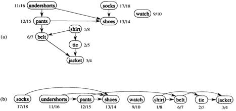
A topological sort of a DAG is a linear ordering of vertices such that if (u, v) in E, then u appears somewhere before v (not like sorting numbers!). The topological sorting algorithm is described below:

TOPOLOGICAL-SORT(V, E)

Call DFS(V, E) to compute finishing times f[v] for all v in V

Output vertices in order of decreasing finish times

It should be clear from above discussion that we don’t need to sort by finish times.

• We can just output vertices as they are finished and understand that we want the reverse of this list.

• Or we can put vertices onto the front of a linked list as they are finished. When done, the list contains vertices in topologically sorted order.

For example, from Figure 4.3.1 the order of vertices:

18 Socks

16 underpants

15 Pants

14 Shoes

10 Watch

8 Shirt

7 Belt

5 Tie

4 jacket

Shortest Paths

A path in a graph is a sequence of vertices in which every two consecutive vertices are connected. If the first vertex of the paths is v and the last is u, we say that the path is a path from v to u. Most of the time, we are interested in paths which do not have repeated vertices. These paths are called simple paths. Since we want to find shortest paths, we define a length of a path as the sum of lengths of its edges.

The shortest path problem is broadly divided into two major versions, the single source shortest path (SSSP) and all pairs shortest paths (APSP). In the SSSP version, given a source vertex s, the goal is to find the shortest paths from s to all other vertices in the graph. In the APSP version, for every pair of vertices (u, v), the goal is to in find the shortest paths between them. Clearly, if we are able to solve SSSP, we are also able to solve APSP by solving SSSP problem for every vertex as the source vertex. While this method is absolutely correct, as we will see, it is not always optimal.

SSSP Problem

Notice that if a graph has uniform length of all edges we already know how to solve the SSSP problem. That is if all edges have the same length, then the shortest path between two vertices is a path which has the fewer number of edges from all such paths and we already know that it can be solved with breadth first search.

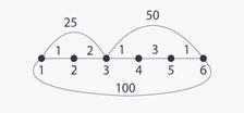
The problem becomes harder if lengths are not uniform, in which case the shortest path may have many more edges that any other path. Consider the graph in Figure 4.3.2 where the edge lengths are shown near the edges. Note that the shortest path between vertex 1 and 6 has length 8 and contains 5 edges, while any other path from vertex 1 to 6 with fewer edges is longer. It is easy to see that BFS does not work.

Figure 4.3.2 : A weighted graph

Having highlighted about the nature of the problem we proceed to describe the solution method. The most famous algorithm for solving the SSSP problem is Dijsktra algorithm. It is based on a crucial assumption that all edges have non-negative weights. Its correct logic strongly depends on this assumption that the algorithm does not work if the graph has negative edges.

Let d(s, v) be the length of shortest path from source vertex s to vertex v. The Dijkstra algorithm partition the set V of vertices into two disjoint sets X := {v : such that d(s, v) has its final value already computed} and V \ X. Initially V \ X is empty and initialize d(s, s):= 0 and d(s, v):= infinity for all v != s. Then as long as V \ X in not empty (i.e., there is at least one vertex v for which d(s, v) is not already computed), repeat the following step.

Let v be a vertex in V \ X such that d(s, v) is minimal from all such vertices. Move v to X and for each edge (v, u) such that v is in V \ X, update the current distance to u, i.e., do d(s, u) = min(d(s, u), d(s, v) + w(v, u)), where w(v, u) is the length of the edge from v to u.

Note that for the Dijkstra algorithm the following invariant holds: As long as V \X in not empty, there exists a vertex v in V \ X such that d(s, v) has already assigned its final value. This is true because we are dealing only with non negative edges and this vertex has to have the minimal value of d(s, v) from all vertices in V \ X.

The time complexity of Dijkstra algorithm is as follows. Note that there are n (number of nodes) iterations of the main loop, because during each iteration one vertex is moved to the set X. Also during iteration a vertex v which has the minimum value of d(s, v) is selected from vertices in V \ X, and the distance value for all neighbours of v is updated. It is easy to see that during the execution, this minimum is selected exactly n times and the distance values is updated exactly m (number of edges) times, because we do it once for every edge. Let f(n) be the time complexity of selecting a minimum and let g(n) be the time complexity of the update operation. Therefore, the total time complexity is O(n * f(n) + m * g(n)).

Both of these functions can be implemented in many different ways. The most common implementation is to use a heap based priority queue with decrease-key operation for updating distance values or to use a balanced binary tree. Both these methods give time complexity O(n log n + m log n). There are many cases that we can do better than that, for example, if length are small integers or if we can use more advanced priority queues like Fibonacci heap. But these methods are beyond the scope of this module; nevertheless it is worth knowing that they exist.

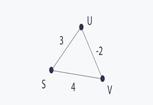
Now observe what can happen in case we have negative length edges. Consider the graph in Figure 4.3.3 . The Dijkstra algorithm does not work because it assigns d(s, s):= 0, then d(s, u):= 3 and finally d(s, v):= 1, but actually there exists a path from s to u of length 2.

Figure 4.3.3 : A negative weighted graph

In this case a different method called Bellman-Ford (BF) algorithm can be used. The idea behind this algorithm is to have computed shortest paths which uses at most k edges in the kth iteration of the algorithm. After n - 1 iterations, all shortest paths are computed, because a simple path in a graph with n vertices can have at most n - 1 edges. The BF algorithm proceeds as shown below:

for v in V:
    if v == s:
        d[v] := 0
    else:
        d[v] := INFINITY
for i = 1 to n - 1:
    for (u, v) in E:
        d[v] := min(d[v], d[u] + length(u, v))

In order to see why the algorithm is correct, notice that if u, ..., w, v is the shortest path from u to v, then it can be constructed from the shortest path from u to w by adding the edge between w and v to it. This is a very important and widely used fact about shortest paths. Bellman-Ford algorithm works for negative edges also. One important assumption is that the input graph cannot contain a negative length cycle since the problem is not well defined in such graphs (you can construct a path of arbitrary small length). In fact, this algorithm can be used to detect if a graph contains a negative length cycle.

The time complexity of Bellman-Ford is O(n * m), because it performs n iterations and in each it examines all edges in the graph. Although this algorithm was invented a long time ago, it is still the fastest strongly polynomial algorithm, i.e., its polynomial complexity depends only on the number of vertices and the number of edges. It is the method commonly used in finding shortest paths in general graphs with arbitrary edges lengths.

APSP Problem

In this version of the problem, we need to find the shortest paths between all pairs of vertices. The most straightforward method to do that is to use any known algorithm for SSSP version of the problem and run it from every vertex as a source. This results in O(n * m log n) time if we use Dijkstra algorithm and O(n2 * m) if we use Bellman-Ford algorithm. If we do not have to deal with negative edges it works well because Dijkstra algorithm is quite fast.

Let us now take a look at Floyd-Warshall (FW) algorithm which runs in O(n3) even if there are negative length edges, which is based dynamic programming. The idea behind the FW algorithm is following: Let d(i, j, k) be the shortest path between vertex i and j which uses only vertices with numbers in {1, 2, ..., k}. Then d(i, j, n) is the desired result which we want to compute for all i and j. Assume that we have computed d(i, j, k) for all i and j, and we want to compute d(i, j, k + 1). Two cases need to be considered, namely, the shortest path between i and j which uses vertices in {1, 2, ..., k + 1} may either use the vertex with number k+1 or not.

If it does not use it, then it is equal to d(i, j, k).

If it uses vertex k+1, it is equal d(i, k + 1, k) + d(k + 1, j, k), since the vertex k+1 can occur only once in such a path.

The Floyd-Warshall algorithm is presented below.

for v in V:
    for u in V:
        if v == u:
            d[v][u] := 0
        else:
            d[v][u] := INFINITY
for (u, v) in E:
    d[u][v] := length(u, v)
for k = 1 to n:
    for i = 1 to n:
        for j = 1 to n:
            d[i][j] = min(d[i][j], d[i][k] + d[k][j])

This algorithm largely uses dynamic programming as it may have been observed. Its running time is O(n3), because it performs n iterations and in each it examines all pairs of vertices. In fact, it can be implemented so that it uses only O(n2) space and the paths can also be reconstructed very fast.

Conclusion

In this activity we presented the topological sort algorithm and algorithms for the shortest path problem. The topological sort takes an acyclic digraph as input and uses the DFS traversal to enumerate nodes in order precedence. We described the Dijkstra algorithm that finds the shortest path for a single source graph with non-negative edge weights, and the Bellman Ford algorithm which also works for graphs with negative edge weights. For the case of multiple sourced graphs, we showed that the two algorithms can be adapted with some loss of efficiency, though. For this reason, the Floyd-Warshall algorithm which finds shortest paths in multiple sourced graphs setting with arbitrary edge weights was discussed.

Assessment

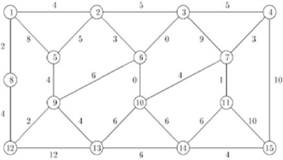
1. Given a weighted graph in Figure 4.3.4 , find the shortest path from point 1 to all other nodes.

Figure 4.3.4 : A weighted graph

Apr 19, 2021, 5:50 PM

Figure 16

2. Show the steps of Bellman-Ford algorithm to find shortest path from A to E using the graph in Figure 4.3.5 . What is the result? How would the Floyd-Warshall algorithm behave when this graph is used as input?

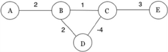
Figure 4.3.5 : A negative weighted graph