17.4: Why Tree Diagrams Work

We’ve now settled into a routine of solving probability problems using tree diagrams. But we’ve left a big question unaddressed: mathematical justification behind those funny little pictures. Why do they work?

The answer involves conditional probabilities. In fact, the probabilities that we’ve been recording on the edges of tree diagrams are conditional probabilities. For example, consider the uppermost path in the tree diagram for the hockey team problem, which corresponds to the outcome \(WW\). The first edge is labeled \(1/2\), which is the probability that the local team wins the first game. The second edge is labeled \(2/3\), which is the probability that the local team wins the second game, given that they won the first—a conditional probability! More generally, on each edge of a tree diagram, we record the probability that the experiment proceeds along that path, given that it reaches the parent vertex.

So we’ve been using conditional probabilities all along. For example, we concluded that:

\[\nonumber \text{Pr}[WW] = \frac{1}{2} \cdot \frac{2}{3} = \frac{1}{3}.\]

Why is this correct?

The answer goes back to Definition 17.2.1 of conditional probability which could be written in a form called the Product Rule for conditional probabilities:

Rule: Conditional Probability Product Rule - 2 Events

\[\nonumber \text{Pr}[E_1 \cap E_2] = \text{Pr}[E_1] \cdot \text{Pr}[E_2 \mid E_1].\]

Multiplying edge probabilities in a tree diagram amounts to evaluating the right side of this equation. For example:

\[\begin{aligned} \text{Pr}&[\text{win first game} \cap \text{win second game}] \\ &= \text{Pr}[\text{win first game}] \cdot \text{Pr}[\text{win second game} \mid \text{win first game}] \\ &= \frac{1}{2} \cdot \frac{2}{3}. \end{aligned}\]

So the Conditional Probability Product Rule is the formal justification for multiplying edge probabilities to get outcome probabilities.

To justify multiplying edge probabilities along a path of length three, we need a rule for three events:

\[\nonumber \text{Pr}[E_1 \cap E_2 \cap E_3] = \text{Pr}[E_1] \cdot \text{Pr}[E_2 \mid E_1] \cdot \text{Pr}[E_3 \mid E_1 \cap E_2].\]

An \(n\)-event version of the Rule is given in Problem 17.1, but its form should be clear from the three event version.

Probability of Size-\(k\) Subsets

As a simple application of the product rule for conditional probabilities, we can use the rule to calculate the number of size-\(k\) subsets of the integers \([1..n]\). Of course we already know this number is \({n \choose k}\), but now the rule will give us a new derivation of the formula for \({n \choose k}\).

Let’s pick some size-\(k\) subset, \(S \subseteq [1..n]\), as a target. Suppose we choose a size-\(k\) subset at random, with all subsets of \([1..n]\) equally likely to be chosen, and let \(p\) be the probability that our randomly chosen equals this target. That is, the probability of picking \(S\) is \(p\), and since all sets are equally likely to be chosen, the number of size-\(k\) subsets equals \(1/p\).

So what’s \(p\)? Well, the probability that the smallest number in the random set is one of the \(k\) numbers in \(S\) is \(k/n\). Then, given that the smallest number in the random set is in \(S\), the probability that the second smallest number in the random set is one of the remaining \(k - 1\) elements in \(S\) is \((k-1)/(n-1)\). So by the product rule, the probability that the two smallest numbers in the random set are both in \(S\) is

\[\nonumber \frac{k}{n} \cdot \frac{k-1}{n-1}.\]

Next, given that the two smallest numbers in the random set are in \(S\), the probability that the third smallest number is one of the \(k - 2\) remaining elements in \(S\) is \((k-2)/(n-2)\). So by the product rule, the probability that the three smallest numbers in the random set are all in \(S\) is

\[\nonumber \frac{k}{n} \cdot \frac{k-1}{n-1} \cdot \frac{k-2}{n-2}.\]

Continuing in this way, it follows that the probability that all \(k\) elements in the randomly chosen set are in \(S\), that is, the probabilty that the randomly chosen set equals the target, is

\[\begin{aligned} p &= \frac{k}{n} \cdot \frac{k-1}{n-1} \cdot \frac{k-2}{n-2} \cdots \frac{k - (k-1)}{n - (k-1)} \\ &= \frac{k \cdot (k-1) \cdot (k-1) \cdots 1}{n \cdot (n-1) \cdot (n-2) \cdots (n-(k-1))} \\ &= \frac{k!}{n!/(n-k)!} \\ &= \frac{k!(n-k)!}{n!}. \end{aligned}\]

So we have again shown the number of size-\(k\) subsets of \([1..n]\), namely \(1/p\), is

\[\nonumber \frac{n!}{k!/(n-k)!}.\]

Medical Testing

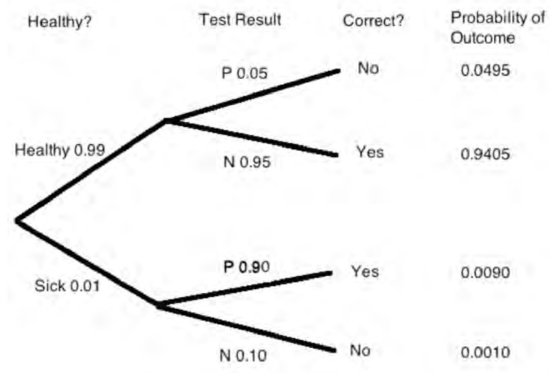
Breast cancer is a deadly disease that claims thousands of lives every year. Early detection and accurate diagnosis are high priorities, and routine mammograms are one of the first lines of defense. They’re not very accurate as far as medical tests go, but they are correct between 90% and 95% of the time, which seems pretty good for a relatively inexpensive non-invasive test.¹ However, mammogram results are also an example of conditional probabilities having counterintuitive consequences. If the test was positive for breast cancer in you or a loved one, and the test is better than 90% accurate, you’d naturally expect that to mean there is better than 90% chance that the disease was present. But a mathematical analysis belies that gut instinct. Let’s start by precisely defining how accurate a mammogram is:

1. If you have the condition, there is a 10% chance that the test will say you do not have it. This is called a “false negative.”
2. If you do not have the condition, there is a 5% chance that the test will say you do. This is a “false positive.”

Four Steps Again

Now suppose that we are testing middle-aged women with no family history of cancer. Among this cohort, incidence of breast cancer rounds up to about 1%.

Step 1: Find the Sample Space

The sample space is found with the tree diagram in Figure 17.2.

Figure 17.2 The tree diagram for a breast cancer test.

Step 2: Define Events of Interest

Let \(A\) be the event that the person has breast cancer. Let \(B\) be the event that the test was positive. The outcomes in each event are marked in the tree diagram. We want to find \(\text{Pr}[A \mid B]\), the probability that a person has breast cancer, given that the test was positive.

Step 3: Find Outcome Probabilities

First, we assign probabilities to edges. These probabilities are drawn directly from the problem statement. By the Product Rule, the probability of an outcome is the product of the probabilities on the corresponding root-to-leaf path. All probabilities are shown in Figure 17.2.

Step 4: Compute Event Probabilities

From Definition 17.2.1, we have

\[\nonumber \text{Pr}[A \mid B] = \frac{\text{Pr}[A \cap B]}{\text{Pr}[B]} = \frac{0.009}{0.009 + 0.0495} \approx 15.4\%\]

So, if the test is positive, then there is an 84.6% chance that the result is incorrect, even though the test is nearly 95% accurate! So this seemingly pretty accurate test doesn’t tell us much. To see why percent accuracy is no guarantee of value, notice that there is a simple way to make a test that is 99% accurate: always return a negative result! This test gives the right answer for all healthy people and the wrong answer only for the 1% that actually have cancer. This 99% accurate test tells us nothing; the “less accurate” mammogram is still a lot more useful.

Natural Frequencies

That there is only about a 15% chance that the patient actually has the condition when the test say so may seem surprising at first, but it makes sense with a little thought. There are two ways the patient could test positive: first, the patient could have the condition and the test could be correct; second, the patient could be healthy and the test incorrect. But almost everyone is healthy! The number of healthy individuals is so large that even the mere 5% with false positive results overwhelm the number of genuinely positive results from the truly ill.

Thinking like this in terms of these “natural frequencies” can be a useful tool for interpreting some of the strange seeming results coming from those formulas. For example, let’s take a closer look at the mammogram example.

Imagine 10,000 women in our demographic. Based on the frequency of the disease, we’d expect 100 of them to have breast cancer. Of those, 90 would have a positve result. The remaining 9,900 woman are healthy, but 5% of them—500, give or take—will show a false positive on the mammogram. That gives us 90 real positives out of a little fewer than 600 positives. An 85% error rate isn’t so surprising after all.

Posteriori Probabilities

If you think about it much, the medical testing problem we just considered could start to trouble you. You may wonder if a statement like “If someone tested positive, then that person has the condition with probability 18%” makes sense, since a given person being tested either has the disease or they don’t.

One way to understand such a statement is that it just means that 15% of the people who test positive will actually have the condition. Any particular person has it or they don’t, but a randomly selected person among those who test positive will have the condition with probability 15%.

But what does this 15% probability tell you if you personally got a positive result? Should you be relieved that there is less than one chance in five that you have the disease? Should you worry that there is nearly one chance in five that you do have the disease? Should you start treatment just in case? Should you get more tests?

These are crucial practical questions, but it is important to understand that they are not mathematical questions. Rather, these are questions about statistical judgements and the philosophical meaning of probability. We’ll say a bit more about this after looking at one more example of after-the-fact probabilities.

The Hockey Team in Reverse

Suppose that we turn the hockey question around: what is the probability that the local C-league hockey team won their first game, given that they won the series?

As we discussed earlier, some people find this question absurd. If the team has already won the tournament, then the first game is long since over. Who won the first game is a question of fact, not of probability. However, our mathematical theory of probability contains no notion of one event preceding another. There is no notion of time at all. Therefore, from a mathematical perspective, this is a perfectly valid question. And this is also a meaningful question from a practical perspective. Suppose that you’re told that the local team won the series, but not told the results of individual games. Then, from your perspective, it makes perfect sense to wonder how likely it is that local team won the first game.

A conditional probability \(\text{Pr}[B \mid A]\) is called a posteriori if event \(B\) precedes event \(A\) in time. Here are some other examples of a posteriori probabilities:

• The probability it was cloudy this morning, given that it rained in the afternoon.
• The probability that I was initially dealt two queens in Texas No Limit Hold ’Em poker, given that I eventually got four-of-a-kind.

from ordinary probabilities; the distinction comes from our view of causality, which is a philosophical question rather than a mathematical one.

Let’s return to the original problem. The probability that the local team won their first game, given that they won the series is \(\text{Pr}[B \mid A]\). We can compute this using the definition of conditional probability and the tree diagram in Figure 17.1:

\[\nonumber \text{Pr}[B \mid A] = \frac{\text{Pr}[B \cap A]}{\text{Pr}[A]} = \frac{1/3 + 1/18}{1/3 + 1/18 + 1/9} = \frac{7}{9}.\]

In general, such pairs of probabilities are related by Bayes’ Rule:

Theorem \(\PageIndex{1}\): Bayes’ Rule

\[\label{17.4.1} \text{Pr}[B \mid A] = \frac{\text{Pr}[A \mid B] \cdot \text{Pr}[B]}{\text{Pr}[A]}\]

Proof

We have

\[\nonumber \text{Pr}[B \mid A] \cdot \text{Pr}[A] = \text{Pr}[A \cap B] = \text{Pr}[A \mid B] \cdot \text{Pr}[B]\]

definition of conditional probability. Dividing by \(\text{Pr}[A]\) gives (\ref{17.4.1}). \(\quad \blacksquare\)

Philosphy of Probability

Let’s try to assign a probability to the event

\[\nonumber [2^{6972607} - 1 \text{ is a prime number}]\]

It’s not obvious how to check whether such a large number is prime, so you might try an estimation based on the density of primes. The Prime Number Theorem implies that only about 1 in 5 million numbers in this range are prime, so you might say that the probability is about \(2 \cdot 10^{-8}\). On the other hand, given that we chose this example to make some philosophical point, you might guess that we probably purposely chose an obscure looking prime number, and you might be willing to make an even money bet that the number is prime. In other words, you might think the probability is \(1/2\). Finally, we can take the position that assigning a probability to this statement is nonsense because there is no randomness involved; the number is either prime or it isn’t. This is the view we take in this text.

An alternate view is the Bayesian approach, in which a probability is interpreted as a degree of belief in a proposition. A Bayesian would agree that the number above is either prime or composite, but they would be perfectly willing to assign a probability to each possibility. The Bayesian approach is very broad in its willingness to assign probabilities to any event, but the problem is that there is no single “right” probability for an event, since the probability depends on one’s initial beliefs. On the other hand, if you have confidence in some set of initial beliefs, then Bayesianism provides a convincing framework for updating your beliefs as further information emerges.

As an aside, it is not clear whether Bayes himself was Bayesian in this sense. However, a Bayesian would be willing to talk about the probability that Bayes was Bayesian.

Another school of thought says that probabilities can only be meaningfully applied to repeatable processes like rolling dice or flipping coins. In this frequentist view, the probability of an event represents the fraction of trials in which the event occurred. So we can make sense of the a posteriori probabilities of the Cleague hockey example of Section 17.4.5 by imagining that many hockey series were played, and the probability that the local team won their first game, given that they won the series, is simply the fraction of series where they won the first game among all the series they won.

Getting back to prime numbers, we mentioned in Section 8.5.1 that there is a probabilistic primality test. If a number \(N\) is composite, there is at least a \(3/4\) chance that the test will discover this. In the remaining \(1/4\) of the time, the test is inconclusive. But as long as the result is inconclusive, the test can be run independently again and again up to, say, 1000 times. So if \(N\) actually is composite, then the probability that 1000 repetitions of the probabilistic test do not discover this is at most:

\[\nonumber \left( \frac{1}{4}\right)^{1000}\]

If the test remained inconclusive after 1000 repetitions, it is still logically possible that \(N\) is composite, but betting that \(N\) is prime would be the best bet you’ll ever get to make! If you’re comfortable using probability to describe your personal belief about primality after such an experiment, you are being a Bayesian. A frequentist would not assign a probability to \(N\)’s primality, but they would also be happy to bet on primality with tremendous confidence. We’ll examine this issue again when we discuss polling and confidence levels in Section 19.5.

Despite the philosophical divide, the real world conclusions Bayesians and Frequentists reach from probabilities are pretty much the same, and even where their interpretations differ, they use the same theory of probability.

¹The statistics in this example are roughly based on actual medical data, but have been rounded or simplified for illustrative purposes.