24.1: Recoding with Simple Operations

Last updated
Save as PDF

Page ID: 88750

\( \newcommand{\vecs}[1]{\overset { \scriptstyle \rightharpoonup} {\mathbf{#1}} } \) \( \newcommand{\vecd}[1]{\overset{-\!-\!\rightharpoonup}{\vphantom{a}\smash {#1}}} \)\(\newcommand{\id}{\mathrm{id}}\) \( \newcommand{\Span}{\mathrm{span}}\) \( \newcommand{\kernel}{\mathrm{null}\,}\) \( \newcommand{\range}{\mathrm{range}\,}\) \( \newcommand{\RealPart}{\mathrm{Re}}\) \( \newcommand{\ImaginaryPart}{\mathrm{Im}}\) \( \newcommand{\Argument}{\mathrm{Arg}}\) \( \newcommand{\norm}[1]{\| #1 \|}\) \( \newcommand{\inner}[2]{\langle #1, #2 \rangle}\) \( \newcommand{\Span}{\mathrm{span}}\) \(\newcommand{\id}{\mathrm{id}}\) \( \newcommand{\Span}{\mathrm{span}}\) \( \newcommand{\kernel}{\mathrm{null}\,}\) \( \newcommand{\range}{\mathrm{range}\,}\) \( \newcommand{\RealPart}{\mathrm{Re}}\) \( \newcommand{\ImaginaryPart}{\mathrm{Im}}\) \( \newcommand{\Argument}{\mathrm{Arg}}\) \( \newcommand{\norm}[1]{\| #1 \|}\) \( \newcommand{\inner}[2]{\langle #1, #2 \rangle}\) \( \newcommand{\Span}{\mathrm{span}}\)\(\newcommand{\AA}{\unicode[.8,0]{x212B}}\)

Consider the following soccer data set called worldcup2019.csv. Each row of this data set represents one player’s performance in a particular 2019 World Cup game. Notice that we have a couple of players with more than one row (Megan Rapinoe and Rose Lavelle), and several rows for the same game (the first four rows are all from the June 28th game, for instance):

last,first,date,inmins,insecs,outmins,outsecs,gls,asst,tkls,shots

Morgan,Alex,28-Jun-2019,0.0,0.0,90.0,0,0,0,0,2,1

Rapinoe,Megan,28-Jun-2019,0.0,0.0,74.0,27.0,2,0,2,3

Press,Christen,28-Jun-2019,74.0,27.0,90.0,0.0,0,0,1,0

Lavelle,Rose,28-Jun-2019,0.0,0.0,90.0,0.0,0,1,3,0

Lavelle,Rose,7-Jul-2019,0.0,0.0,90.0,0.0,1,0,4,1

Rapinoe,Megan,7-Jul-2019,0.0,0.0,83.0,16.0,1,1,3,2

Lloyd,Carli,7-Jul-2019,83.0,16.0,90.0,0.0,0,0,1,0

Dunn,Crystal,23-Jun-2019,42.0,37.0,81.0,5.0,0,1,1,2

The data set doesn’t really have a meaningful index column, since none of the columns are expected to be unique. So we’ll leave off the “.set_index()” method call when we read it in to Python:

Code \(\PageIndex{1}\) (Python):

wc = pd.read_csv('worldcup2019.csv')

print(wc)

Output:

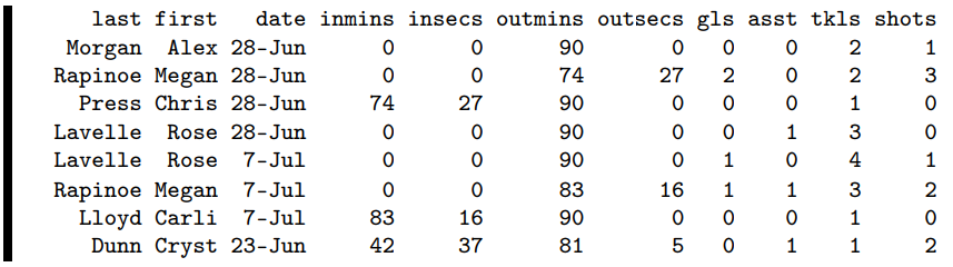
Let’s zero in on the columns with mins and secs in the names. These columns show us the minute and second that the player went in to the game, and the minute and second that they came out. For example, Alex Morgan played the entire 90-minute match on June 28th. Rapinoe started that game, but came out for a substitute at the 74:27 mark. Who replaced her? Looks like Christen Press did, since she entered the game at exactly the same time. In most rows, the player either started the game, or ended the game or both, but the last row (Crystal Dunn’s June 23rd performance) has her entering at 42:37 and exiting at 81:05.

Now the reason I bring this up is because one aspect of our analysis might be computing statistics per minute that each athlete played. If one player scored 3 goals in 200 minutes, for example, and another scored 3 goals in just 150 minutes, we could reasonably say that the second player was a more prolific scorer in that World Cup.

This is hard to do with the data in the form that it stands. So we’ll recode a few of the columns. Let’s collapse the minutes and seconds for each of the two clock times into a single value, in minutes. For readability, we’ll also round this number to two decimal places using the round() function we met on p. 237:

Code \(\PageIndex{2}\) (Python):

wc['intime'] = np.round(wc['inmins'] + (wc['insecs']/60),2)

wc['outtime'] = np.round(wc['outmins'] + (wc['outsecs']/60),2)

We’re taking advantage of vectorized operations here. For each row, we need to divide the insecs value by 60 (to convert it to minutes) and add it to the inmins value. Pandas makes this super easy here, since we can just write out those operations once, and it will compute it for every single row!

Let’s delete the old, superfluous columns now and looksie:

Code \(\PageIndex{3}\) (Python):

del wc['inmins']

del wc['insecs']

del wc['outmins']

del wc['outsecs']

print(wc)

This is much less unwieldy (more wieldy?) than dealing with minutes and seconds separately.

(Incidentally, notice that the technique presented here creates new columns (with new names) and then deletes the old columns. I strongly recommend doing it this way. If you try to change the values of an existing DataFrame column, Pandas will often give you a strange-looking message informing you of a “SettingWithCopyWarning”. The meaning is a bit esoteric, but in layman’s terms it means “your operation may not have actually worked.” Avoid this problem by creating new columns instead.)