24.2: Transforming with Simple Operations

Last updated
Save as PDF

Page ID: 88751

\( \newcommand{\vecs}[1]{\overset { \scriptstyle \rightharpoonup} {\mathbf{#1}} } \) \( \newcommand{\vecd}[1]{\overset{-\!-\!\rightharpoonup}{\vphantom{a}\smash {#1}}} \)\(\newcommand{\id}{\mathrm{id}}\) \( \newcommand{\Span}{\mathrm{span}}\) \( \newcommand{\kernel}{\mathrm{null}\,}\) \( \newcommand{\range}{\mathrm{range}\,}\) \( \newcommand{\RealPart}{\mathrm{Re}}\) \( \newcommand{\ImaginaryPart}{\mathrm{Im}}\) \( \newcommand{\Argument}{\mathrm{Arg}}\) \( \newcommand{\norm}[1]{\| #1 \|}\) \( \newcommand{\inner}[2]{\langle #1, #2 \rangle}\) \( \newcommand{\Span}{\mathrm{span}}\) \(\newcommand{\id}{\mathrm{id}}\) \( \newcommand{\Span}{\mathrm{span}}\) \( \newcommand{\kernel}{\mathrm{null}\,}\) \( \newcommand{\range}{\mathrm{range}\,}\) \( \newcommand{\RealPart}{\mathrm{Re}}\) \( \newcommand{\ImaginaryPart}{\mathrm{Im}}\) \( \newcommand{\Argument}{\mathrm{Arg}}\) \( \newcommand{\norm}[1]{\| #1 \|}\) \( \newcommand{\inner}[2]{\langle #1, #2 \rangle}\) \( \newcommand{\Span}{\mathrm{span}}\)\(\newcommand{\AA}{\unicode[.8,0]{x212B}}\)

Now that we’ve converted the awkward minutes-and-seconds columns to just “time” columns, all we need to do to complete our analysis is transform this data by computing a new quantity entirely: the total number of minutes played for each player in each game. Again, Pandas makes this easy:

Code \(\PageIndex{1}\) (Python):

wc['minsplayed'] = wc.outtime - wc.intime

print(wc)

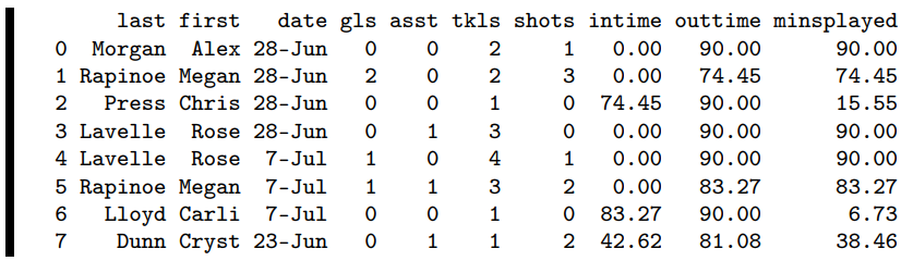
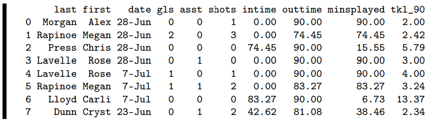
Voilà. We now have the time-on-field for each player, which gives us a whole new avenue of exploration. For example, any of the counting stats (goals, assists, etc.) can be converted into a “perminute” version, showing us how productive a player was while on the field. Let’s do that for tkls (“tackles”), and multiply by 90 to obtain a “tackles-per-90-minutes” statistic¹ :

Code \(\PageIndex{2}\) (Python):

wc['minsplayed'] = wc['outtime'] - wc['intime']

wc['tkl_per_90'] = np.round(wc['tkls'] /

wc['minsplayed'] * 90,2)

del wc['tkls']

Transforming Grouped Data

The above example computed tackles-per-game all right, but it still left us with one row for every player-performance. (In other words, the results had two rows for Rose Lavelle, one giving her tkl_per_90 for the June 28th game, and one giving it for the July 7th game.)

We might instead be interested in a player-by-player analysis: overall in the entire month-long World Cup, which players had the most tackles-per-game? This is easy to do with the .groupby() method that we first encountered in section 18.2 (p. 189). First, we group the rows by the first two columns (since first-and-last-namestogether are needed to uniquely identify a single player):

Code \(\PageIndex{3}\) (Python):

grouped_wc = wc.groupby(['last','first'])

We then take our new, temporary grouped_wc variable and extract the gls, asst, shots, tkls, and minsplayed columns from it, summing each of them to produce the per-player values in the result:

Code \(\PageIndex{4}\) (Python):

by_player = grouped_wc.sum()

This yields:

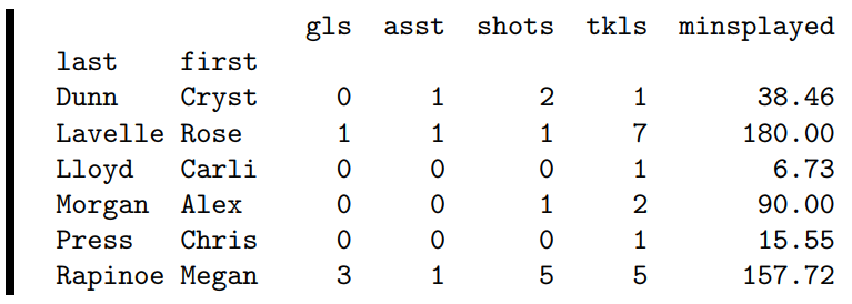
Now, we’re ready to compute a per-game analysis as before, but this time for each player’s entire World Cup games:

Code \(\PageIndex{5}\) (Python):

by_player['tkl_per_90'] = (np.round(by_player['tkls'] / by_player['minsplayed'] * 90,2))

del by_player['tkls']

¹I’m choosing 90 minutes here because that’s how long a regulation-length soccer match is. Therefore, our new tkl_per_90 column gives us “numberof-tackles-per-complete-game,” which is easier to interpret than “tackles-per-minute,” which would be a miniscule number for any player.