24.3: More Complex Transformations

In all the above examples, we took advantage of Pandas vectorized operations. With just a single line of code like “wc['minsplayed'] = wc.outtime - wc.intime”, we could compute our entire new transformed column in one fell swoop.

Sometimes, we’re not so lucky. In particular, if the computation of the transformed column is more complicated than just numeric operations – like, if it involves branches, loops, or calling other functions – we normally can’t compute it all at once. Instead, we have to resort to a loop.

Pandas makes this procedure a bit awkward in my opinion. But once you learn the pattern, it’s not hard to imitate. Here’s the pattern for creating a transformed/recoded column that requires more complex operations:

1. Create a function that will compute the transformed value for a single row. Its arguments should be whatever column values are necessary to derive the new value, and its return value should be the desired transformation.
2. Create an empty NumPy array to hold the row-by-row results, and make sure it’s the right type.
3. Write a loop that will iterate through all the rows of the original DataFrame. For each row, pass the appropriate values to the function, and then append the return value to the evergrowing NumPy array.
4. Finally, slap that NumPy array on to the DataFrame as a new column.

Here’s a couple examples. First, suppose we want to compute a shooting percentage for each player; in other words, how many goals they scored per shot they took. Now you might think we could simply use vectorized operations:

Code \(\PageIndex{1}\) (Python):

wc['shots_per_goal'] = wc.gls / wc.shots

The problem is, for players who never attempted a shot in the game, this would result in dividing by zero, a cardinal sin. Sports convention says that if a player makes 0 goals in 0 attempts, their shooting percentage is 0.00, even though mathematically-speaking this is undefined.

Very well, following our procedure from above, we’ll first define a function shooting_perc():

Code \(\PageIndex{2}\) (Python):

def shooting_perc(gls, shots):

if shots == 0:

return 0.0

else:

return np.round(gls / shots * 100, 1)

Then, we create an empty NumPy array. Here’s how:

Code \(\PageIndex{3}\) (Python):

s_perc = np.array([])

Looks weird, I know. But remember, the array() function (review p. 63) takes a boxie-enclosed list of elements. If we enclose nothing inside the boxies, that effectively makes it an empty list.

And why would we want to do that? Because we need to continually add to this array, one value for each row in the DataFrame. At the end, there must be exactly as many elements in s_perc as there are rows in wc, otherwise we won’t be able to add it as a new column.

Here’s the loop (step 3 from the shaded box):

Code \(\PageIndex{4}\) (Python):

for row in wc.itertuples():

new_s_perc = shooting_perc(row.gls, row.shots)

s_perc = np.append(s_perc, new_s_perc)

I’ve chosen to create a temporary variable here (new_s_perc) for readability. The first line of the loop body says to take the current row’s gls and shots values, and send them as arguments to the shooting_perc() function. That function, which we defined above, will return us a single number which is the shooting percentage for that row. The second line then appends that single new_s_perc value to the end of the ever-growing s_perc array.

Finally, we add this new column to the wc DataFrame proper:

Code \(\PageIndex{5}\) (Python):

wc['s_perc'] = s_perc

which gives us:

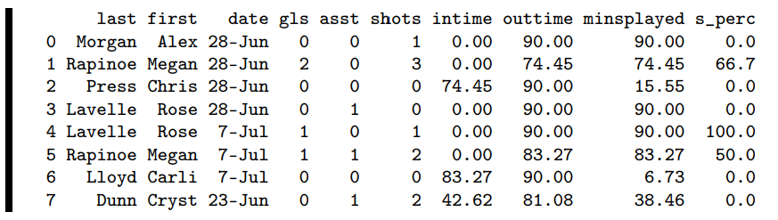
Rose Lavelle’s July 7th game was the only perfect shooting performance in this data set – who knew?

We’ll complete this chapter with a slightly more complex example, but which still follows the shaded box pattern.

Say we’re also interested in which players started which games (as opposed to being a mid-game substitute). Obviously, a starter is someone who entered the game at time 0. To create a new column for this, we’ll need our function to return the boolean value True if the player’s intime value was zero, and False otherwise. Here’s the complete code snippet for this transformation:

Code \(\PageIndex{6}\) (Python):

def starter_func(intime):

if intime == 0:

return True

else:

return False

starter = np.array([]).astype(bool)

for row in wc.itertuples():

starter = np.append(starter, starter_func(row.intime))

wc['starter'] = starter

Output:

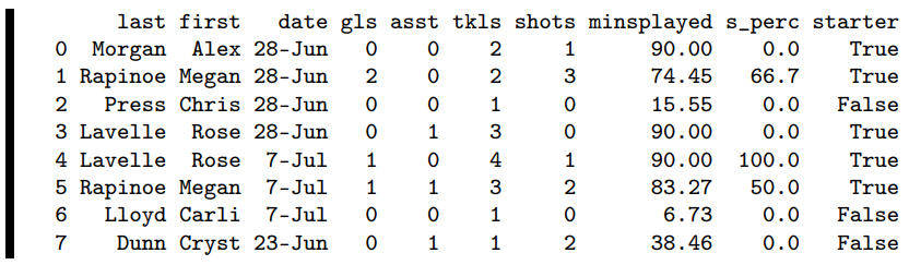
One subtle point that is easy to miss: when we first created the empty starter array, we typed “.astype(bool)” at the end. This is because by default, the values of a new empty array will be floats. This worked fine for the shooting percentage example, because that’s actually what we wanted, but here we want True/False values instead (for “starter” and “non-starter.”)

Pretty cool, huh? The original DataFrame had the information we wanted, but not in the form we really needed it. What we wanted was not the entry time and exit time of each player (both in minutes and seconds) but rather the total time that player was on the pitch, and whether or not they started the game. We also wanted to convert several of the raw statistics into per-complete game numbers, and to compute meaningful ratios like shooting percentage or fouls per assist.

Recoding and transforming turn out to be common tasks for a simple reason: whoever collects a data set can rarely predict how an analyst will eventually use it. We’re very grateful to the author of the .csv file, since it contains the raw material we need to evaluate our team’s performances; but how were they to know that length-of-time-on-the-field and who-started-which-game was going to be important to us? They couldn’t. But thanks to recoding and transformation skills, we can cope.