4.7: Smooth Air-Gap Synchronous Machine Model

A specific result in this section is the terminal relations that constitute the lumped-parameter model for a three-phase two-pole smooth air-gap synchronous machine. The derivations are aimed at exemplifying the pattern that can be followed in describing a wide class of magnetic field devices modeled by coupling at surfaces.

In the cross-sectional view of the smooth air-gap machine shown in Fig. 4.7.1a, the stator structure consists of a laminated circular cylindrical material having permeability \(\mu_s\) with outside radius \(a\) and inner radius \(b\). Imbedded in slots on this inner surface are three windings, having turns densities that vary sinusoidally with \(\theta\). These slots are typically as shown in Fig. 4.7.2b, where the laminations used for construction of rotor and stator for the generator of Fig. 4.7.2a are pictured. Only one of these stator windings is shown in Fig. 4.7.1, the "a" phase with its magnetic axis at \(\theta =-90^{o}\). The "b" and "c" phases are similarly distributed but rotated so that their magnetic axes are respectively at the angles \(30^{o}\) and \(150^{o}\). Thus the peak surface current density for the respective windings comes at the angles \(\theta = 0^{0}, \theta = 120^{o}\), and \( \theta = 240^{o}\). These stator windings have peak turns densities \(N_a, N_b, N_c\), respectively, and carry the terminal currents \((i_a, i_b, i_c)\). Because the stator windings essentially form a current sheet at the radius \(b\), their contribution to the field is modeled by the surface current density

\[ \begin{align} K_z^2 &= i_a (t) N_a \, cos(\theta) + i_b (t) N_b \, cos(\theta - \frac{2 \pi}{3}) + i_c (t) N_c \, cos (\theta - \frac{4 \pi}{3}) \nonumber \\ &= Re \, \tilde{K}^s e^{-j \theta}; \quad \tilde{K}^s = i_a N_a +i_bN_b e^{j (\frac{2 \pi}{3})} + i_c N_c e^{j (\frac{4 \pi}{3})} \nonumber \end{align} \label{1} \]

There is only one phase on the rotor, consisting of sinusoidally distributed windings of peak turns density \(N_r\) excited through slip rings by the terminal current \(i_r\). With the rotor angular position denoted by \(\theta_r\), the rotor current is modeled by a surface current density at \(r = c\) of

\[ K_z^r = i_r (t) N_r \, cos(\theta - \theta_r) = Re \tilde{K}^r e^{-j \theta}; \quad \tilde{K}^r = i_r N_r e^{j \theta_r} \label{2} \]

These excitations have been written in the complex amplitude notation. Fields in each region are described by the polar coordinate transfer relations of Table 2.19.1 with \(m = 1\).

The objective in the following calculations is to relate the electrical and mechanical terminal relations so that electromechanical coupling, represented schematically in Fig. 4.7.3, is specified in the form

\[\begin{bmatrix} \lambda_a \\ \lambda_b \\ \lambda_c \\ \lambda_r \end{bmatrix} = \begin{bmatrix} L_{aa} & L_{ab} & L_{ac} & L_{ar} \\ L_{ba} & L_{bb} & L_{bc} & L_{br} \\ L_{ca} & L_{cb} & L_{cc} & L_{cr} \\ L_{ra} & L_{rb} & L_{rc} & L_{rr} \end{bmatrix} \begin{bmatrix} i_a \\ i_b \\ i_c \\ i_r \end{bmatrix} \label{3} \]

\[ \tau_z = \tau_z (i_a, i_b, i_c, i_r, \theta_r) \label{4} \]

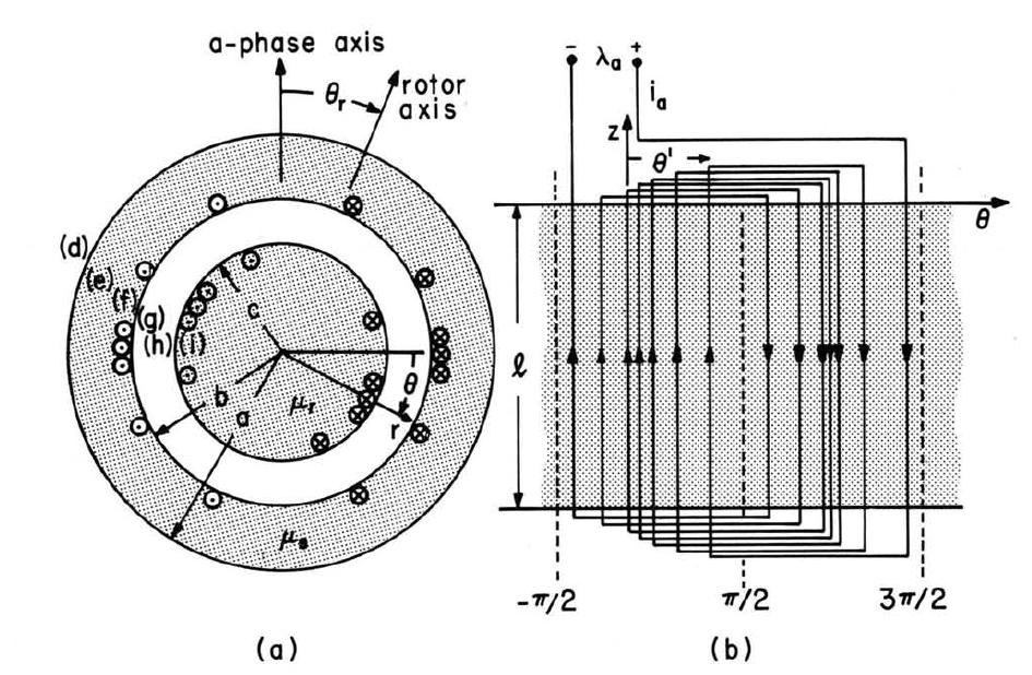
Fig.4.7.1.(a)Cross-sectional view of smooth air-gap synchronous machine showing only one of three phases on stator.(b)Distribution of"a"-phase windings on stator as seen looking radially inward.

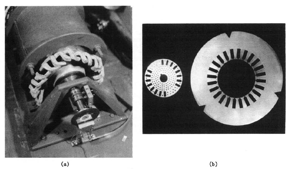
Fig.4.7.2 (a)Model synchronous alternator having rating of about one kVA and modeling 900 MVA machine. Unit is one of several used in MIT Electric Power Systems Engineering Laboratory as part of model power system. Slip rings for supplying field current are on shaft near bearing. Disk with holes is for measurement of angular position of rotor (b)Rotor and stator laminations used for model machine of (a). Rectangular slots carry windings. Conducting rods inserted through the circular holes in the rotor are shorted at the ends of the rotor to simulate transient eddy-current (induction machine) effects in full-scale machine. The scaling requires that the model have extremely narrow air gap of about 0.23mm,as compared to the gap of about 7 cm in the full-scale machine.

Boundary Conditions

The field excitations represented by Eqs. \ref{1} and \ref{2}, written in complex-amplitude notation, can be matched by single components of the fields represented in each region by the polar coordinate transfer relations of Table 2.19.1. In view of the \(\theta\) dependence of the current sheets, \(m = 1\).

Fig. 4.7.1.

Positions adjacent to the boundaries between current-free regions of uniform permeability in Fig. 4.7.1a are denoted by (d) - (i). Fields are assumed to vanish far from the outer surface. At each surface, the normal flux density is continuous (Eq. 2.10.22). This means that the vector potential is continuous, and hence

\[ \tilde{A}^d = \tilde{A}^e \label{5} \]

\[ \tilde{A}^f = \tilde{A}^g \label{6} \]

\[ \tilde{A}^h = \tilde{A}^i \label{7} \]

The jump in the tangential field is equal to the surface current density (Eq. 2.10.21), and hence

\[ \tilde{H}^d_{\theta} - \tilde{H}^e_{\theta} = 0 \label{8} \]

\[ \tilde{H}^f_{\theta} - \tilde{H}^g_{\theta} = \tilde{K}^s \label{9} \]

\[ \tilde{H}^h_{\theta} - \tilde{H}^i_{\theta} = \tilde{K}^r \label{10} \]

Bulk Relations

Each of the uniform regions is described by Eq. (c) of Table 2.19.1. In the exterior region, \(\alpha \rightarrow \infty\), \(\beta = a\), and \(\mu = \mu_o\)

\[ \tilde{H}_{\theta}^d = \frac{1}{\mu_o} f_1 (\infty, a) \tilde{A}^d \label{11} \]

In the stator, \(\alpha = a\), \(\beta = b\), and \(\mu = \mu_s\):

\[\begin{bmatrix} \tilde{H}^{e}_{\theta} \\ \tilde{H}^{f}_{\theta} \end{bmatrix} = \frac{1}{\mu_s} \begin{bmatrix} f_1(b,a) & g_1(a,b) \\ g_1(b,a) & f_1(a,b) \end{bmatrix} \begin{bmatrix} \tilde{A}^e \\ \tilde{A}^f \end{bmatrix} \label{12} \]

In the air gap, \(\alpha = b\), \(\beta = c\), and \(\mu = \mu_o\):

\[\begin{bmatrix} \tilde{H}^{g}_{\theta} \\ \tilde{H}^{h}_{\theta} \end{bmatrix} = \frac{1}{\mu_o} \begin{bmatrix} f_1(c,b) & g_1(b,c) \\ g_1(c,b) & f_1(b,c) \end{bmatrix} \begin{bmatrix} \tilde{A}^g \\ \tilde{A}^h \end{bmatrix} \label{13} \]

and finally, in the rotor, \(\alpha = c\), \(\beta = 0\), and \(\mu = \mu_r\):

\[ \tilde{H}_{\theta}^i = \frac{1}{\mu_r} f_1(0,c) \tilde{A}^i \label{14} \]

Torque as a Function of Terminal Currents and Rotor Angle

With the surface of integration for the stress tensor just inside the stator, it follows from Eq. 4.2.3 that the rotor torque is

\[ \tau_z = (2 \pi b^2 l) \frac{1}{2} Re \big [ (\tilde{H}_{\theta}^g)^{*} \tilde{B}_r^g \big] = \pi b^2 l Re \big [ (\tilde{H}_{\theta}^g)^{*} (\frac{-j \tilde{A}^g}{b}) \big] \label{15} \]

It will be seen shortly that the electrical terminal relations can be computed from \(\tilde{A}^g\). It is therefore convenient to also express Equation \ref{15} in terms of \(\tilde{A}^g\) and the given surface currents. To this end, Eqs. \ref{5} and \ref{8} are used to replace (d)-(e) in Equation \ref{11}, while Eqs. \ref{6} and \ref{9} are used to replace \(\tilde{H}^f_{\theta}\) and \(\tilde{A}^f\) in Equation \ref{12} b. Thus, Eqs. \ref{12} can be solved for \(\tilde{H}^g_{\theta}\) as a function of \(\tilde{K}^s\) and \(\tilde{A}^g\):

\[ \tilde{H}_{\theta}^g = - \tilde{K}^s + \frac{\tilde{A}^g}{\mu_s} \Bigg \{ f_1(a,b) + \frac{ g_1(b,a) g_1(a,b)}{ \Big [ \frac{\mu_s}{\mu_o} f_1(\infty,a) - f_1(b,a) \Big ]} \Bigg \} \label{16} \]

Because the geometric quantity multiplying \(\tilde{A}^g\) is real, it is clear that substitution of Equation \ref{16} into Equation \ref{15} gives only

\[ \tau_z = \pi b l R e [ (\tilde{K}^s)^{*} j \tilde{A}^g] \label{17} \]

To evaluate \(\tilde{A}^g\) in terms of \(\tilde{K}^s\) and \(\tilde{K}^r\) (and hence in terms of the terminal currents and \(\theta_r\) ), Eqs. \ref{7} and \ref{10} are used in Equation \ref{14}, which is solved for \(\tilde{H}^h\). This latter quantity is substituted into Equation \ref{13} b. Simultaneous solution of Eqs. \ref{13} then gives a second expression for \(\tilde{H}^g_{\theta}\):

\[ \tilde{H}_{\theta}^g = \frac{\tilde{K}^r g_1(b,c)}{f_1(b,c) - \frac{\mu_o}{\mu_r} f_1(0,c)} + \frac{\tilde{A}^g}{\mu_o} \Bigg \{ f_1(c,b) + \frac{g_1(b,c) g_1(c,b)}{\frac{\mu_o}{\mu_r} f_1(0,c) - f_1(b,c)} \Bigg \} \label{18} \]

By equating Eqs. \ref{16} and \ref{18}, it is now possible to solve for \(\tilde{A}^g\) in terms of the surface currents:

\[ \tilde{A}^g = \frac{\mu_o}{D} \tilde{K}^s + \frac{ \mu_o g_1(b,c)}{d [ f_1(b,c) - \frac{\mu_o}{\mu_r} f_1 (0,c) ]} \tilde{K}^r \label{19} \]

where

\[ D \equiv \frac{\mu_o}{\mu_s} \Bigg \{ f_1(a,b) + \frac{ g_1(b,a) g_1(a,b)}{ \Big [ \frac{\mu_s}{\mu_o} f_1(\infty,a) - f_1(b,a) \Big ] } \Bigg \} - \Bigg \{ f_1(c,b) + \frac{ g_1(b,c) g_1(c,b)}{ \Big [ \frac{\mu_o}{\mu_r} f_1(0,c) - f_1(b,c) \Big ] } \Bigg \} \nonumber \]

A methodical approach to solving the boundary and bulk relations is suited to those comfortable with the reduction of determinants or inclined to use matrix computations. Following this alternative, the boundary conditions, Eqs. \ref{5} to \ref{10}, are used to eliminate the "d", "f", and "i" variables in the bulk relations, Eqs. \ref{11} to \ref{14}. These latter equations are then written in the form

\[\begin{bmatrix} -1 & \frac{1}{\mu_o} f_1 (\infty,a) & 0 & 0 & 0 & 0 \\ -1 & \frac{1}{\mu_s} f_1 (b,a) & 0 & \frac{1}{\mu_s} g_1 (a,b) & 0 & 0 \\ 0 & \frac{1}{\mu_s} g_1 (b,a) & -1 & \frac{1}{\mu_s} f_1 (a,b) & 0 & 0 \\ 0 & 0 & -1 & \frac{1}{\mu_o} f_1 (c,b) & 0 & \frac{1}{\mu_o} g_1 (b,c) \\ 0 & 0 & 0 & \frac{1}{\mu_o} g_1 (c,b) & -1 & \frac{1}{\mu_o} f_1 (b,c) \\ 0 & 0 & 0 & 0 & -1 & \frac{1}{\mu_r} f_1 (0,c) \end{bmatrix} \begin{bmatrix} \tilde{H}_{\theta}^e \\ \tilde{A}^e \\ \tilde{H}_{\theta}^g \\ \tilde{A}^g \\ \tilde{H}_{\theta}^h \\ \tilde{A}^h \end{bmatrix} = \begin{bmatrix} 0 \\ 0 \\ \tilde{K}^s \\ 0 \\ 0 \\ -\tilde{K}^r \end{bmatrix} \label{20} \]

Cramer's rule is then used to deduce \(\tilde{A}^g\), Equation \ref{19}.

Substitution of Equation \ref{19} into the torque expression, Equation \ref{17}, shows that

\[ \tau_z = \frac{\pi b l \mu_o}{D [f_1(b,c) - \frac{\mu_o}{\mu_r} f_1(0,c)]} \, Re [j \tilde{K}^r (\tilde{K}^s)^{*}] \label{21} \]

It follows from Eqs. \ref{1} and \ref{2} that the torque, expressed in terms of the terminal currents, is

\[ \tau_z = \frac{-\pi b l \mu_o g_1(b,c)}{D [f_1(b,c) - \frac{\mu_o}{\mu_r} f_1(0,c)]} \, i_r N_r [i_a N_a \, sin \, \theta_r + i_b N_b \, sin \, (\theta_r - \frac{2 \pi}{3}) + i_c N_c \, sin \, (\theta_r - \frac{4 \pi}{3}) ] \label{22} \]

Electrical Terminal Relations

The flux linked by one turn of the "a"-phase coil running in the +z direction at \(\theta = theta^{'}\) and returning in the -z direction at \(\theta = \theta^{'} + \pi \) is

\[ \phi_{\lambda} = l [A(b,\theta^{'}) - A(b,\theta^{'} + \pi)] = l Re \tilde{A}^g [ e^{-j \theta^{'}} - e^{-j(\theta^{'} + \pi)}] \label{23} \]

Here, use has been made of the relation between the vector potential and the flux, as described in Sec. 2.18 (Eq. (f) of Table 2.18.1).

The flux linked by the turns in the azimuthal interval \(bd \theta^{'}\) is then \(\phi_{\lambda} (bd \theta^{'} N_a \, cos \, \theta^{'})\), and the total flux linked by the "a" phase is

\[ \lambda_a = -blN_a \int_{-\pi/2}^{\pi/2} Re \frac{1}{2} [ e^{j \theta^{'}} + e^{-j \theta^{'}}] \tilde{A}^g [ e^{j \pi} - 1] e^{j \theta^{'}} d \theta^{'} = lb N_a \pi Re \tilde{A}^g \label{24} \]

Substitution of \(\tilde{A}^g\) from Equation \ref{19} and the surface currents from Eqs. \ref{1} and \ref{2} then gives the terminal relation for the "a" phase, in the form of Equation \ref{3} a, where

\[ L_{aa} = \frac{\pi l b \mu_o N_a^2}{D}, \, L_{ab} = - \frac{\pi l b \mu_o N_a N_b}{2D}, \, L_{ac} = - \frac{\pi l b \mu_o N_a N_c}{2D}, \, L_{ar} = L_o l bN_a N_r \, cose \, \theta_r; \nonumber \]

\[ L_o \equiv \frac{\pi \mu_o g_1(b,c)}{D [ f_1(b,c) - \frac{\mu_o}{\mu_r} f_1(0,c) ] } \label{25} \]

By symmetry, the inductances for the "b" and "c" phases are obtained without carrying out the evaluation by simply replacing indices in Equation \ref{25}. For the "b" phase, replace indices \(a \rightarrow b\), \(b \rightarrow a\), \(c \rightarrow a\), and \(\theta_r \rightarrow \theta_r - \frac{2 \pi}{3}\) and for the "c" phase, \(a \rightarrow c\), \(b \rightarrow a\), \(c \rightarrow b\) and \(\theta_r \rightarrow \theta_r - \frac{4 \pi}{3} \).

The remaining flux linkage, \(\lambda_r\), is computed by first recognizing that the flux linked by one turn on the rotor winding running in the z direction at \(\theta^{'}\) and returning at \(\theta^{'} + \pi\) is

\[ \phi_{\lambda} = - lRe \tilde{A}^h [ e^{j \pi} - 1 ] e^{-j \theta^{'}} \label{26} \]

Hence, the total flux linking the rotor winding is

\[ \lambda_r = \int_{\theta_r - \frac{\pi}{2}}^{\theta_r + \frac{\pi}{2}} N_r \, cos (\theta^{'} - \theta_r) \phi_{\lambda} c d \theta^{'} = N_r c l \pi Re \tilde{A}^h e^{j \theta_r} \label{27} \]

The vector potential amplitude required to evaluate this expression follows from Eqs. \ref{7}, \ref{10}, \ref{13} b, and \ref{14}:

\[ \tilde{A}^h = \frac{g_1(c,b) \tilde{A}^g - \mu_o \tilde{K}^r}{ \frac{\mu_o}{\mu_r} f_1(0,c) - f_1(b,c)} \label{28} \]

where \(\tilde{A}^g\) is again Equation \ref{19}, and the surface currents are evaluated in terms of theterminal currents using Eqs. \ref{1} and \ref{2}. Thus, with the use of the transfer function reciprocity relation, \(cg_1(c,b) = -bg_1(b,c)\), Eq. 2.17.10,

\[ L_{ra} = L_o l b N_r N_a \, cos \, \theta_r, \, L_{rb} = L_o l b N_r N_b \, cos(\theta_r - \frac{2 \pi}{3}), \, L_{rc} = L_o l b N_r N_c \, cos( \theta_r - \frac{4 \pi}{2}) \nonumber \]

\[ L_{rr} = L_o l b N_r^2 \Bigg \{ \frac{g_1(b,c)}{D [f_1(b,c) - \frac{\mu_o}{\mu_r} f_1(0,c)]} - \frac{1}{g_1(c,b)} \Bigg \} \label{29} \]

Energy Conservation

Because the electromechanical coupling network represented by Fig. 4.7.3 isconservative, there is considerable redundancy in the terminal relations that have been derived. Con-servation of energy requires that (Eq. 3.5.7 applied to a magnetic system)

\[ \delta w^{'} = \lambda_a \delta i_a + \lambda_b \delta i_b + \lambda_c \delta i_c + \lambda_r \delta i_r + \tau_z \delta \theta_r \label{30} \]

From the assumption that \(w^{'}\) is a state function, it follows that (see Eq. 3.5.4)

\[ \lambda_k = \frac{\partial{w^{'}}}{\partial{i_k}}; \quad k = a,b,c,r; \quad \tau_z = \frac{\partial{w^{'}}}{\partial{\theta_r}} \label{31} \]

Lumped-parameter reciprocity conditions are generated by taking cross-derivatives of these relations:

\[ \frac{\partial{\lambda_k}}{\partial{i_l}} = \frac{\partial{\lambda_l}}{\partial{i_k}}; \quad \frac{\partial{\tau_z}}{\partial{i_k}} = \frac{\partial{\lambda_l}}{\partial{\theta_r}}; \quad \begin{cases} k = a,b,c,r \\\\ l = a,b,c,r \end{cases} \label{32} \]

The four relations among the electrical terminal variables show that

\[ L_{kl} = L_{lk} \label{33} \]

and these conditions are met by the results summarized by Eqs. \ref{25} and the subsequent substitution of indices and Equation \ref{29}. The reciprocity conditions between the torque and the flux linkages, Equation \ref{32}, is also satisfied by Eqs. \ref{22} and Eqs. \ref{25} and \ref{29}. Note that to make it clear that the lumped-parameter reciprocity relations are satisfied, the reciprocity condition for the air-gap transfer relations was used in writing Equation \ref{29}.