
4.10: D-C Magnetic Machines
- Page ID
- 43855
The wide use of the d-c rotating machine justifies the model development undertaken in this section. But, these devices are also a prototype for a family of "conduction" machines which includes the homopolar generator\(^1\) and magnetohydrodynamic energy convertors, to be taken up in Chapter 9. Analogous electric field devices are the Van de Graaff generator, considered in Sec. 4.14, and electro-as dynamic pumps and generators, described in Chaps. 5 and 9.
The developed model for the d-c machine given in Sec. 4.3 (Table 4.3.1, Part 3) is given a more complete characterization in Figs. 4.10.1 through 4.10.4. What is by convention termed the "field" winding is on the stator, which consists of a highly permeable structure wound with a total of \(2n_f\) turns excited through the terminal pair \((i_f,v_f)\). The "armature" is the rotor, with a winding connected through the commutator to the terminal pair \((i_a,v_a)\), so that the distribution of current is essentially stationary in space. The \(\theta\) dependence is shown in Fig. 4.10.2. The rotor core, like the stator magnetic circuit, is modeled here as being infinitely permeable.
With the assumption that the stator is infinitely permeable, it is clear that the magnetic potential on the stator surface, \(\psi^f\), is constant for those points at \(r = R_o\) contiguous with the stator. Integration of Ampere's integral law, Eq. 2.7.1b, over any contour passing between the pole faces through the field winding and closing through the air gap shows that the pole faces differ in \(\psi\) by \(2n_f i_f\). The horizontal mid-plane is defined as the reference \(\psi = 0\). As an approximation that specifies the fringing field in the ranges of \(\theta\) between pole faces, the magnetic potential is taken as the linear interpolation shown in Fig. 4.10.2a. Because the rotor is modeled as infinitely permeable, the tangential magnetic field at the rotor surface is equal to the surface current density \(K_z\), as shown in Fig. 4.10.2b (an application of Eq. 2.10.21). The number of turns per unit azimuthal length on the rotor is \(N_a\).
The commutator, which consists of conducting segments that are sequentially connected to the armature terminals through brushes, as shown in Fig, 4.10.3a,\(^2\) is attached to one end of the rotor. Thus it rotates with the same angular velocity \(\Omega\) (defined as positive in the positive \(\theta\) direction) as the rotor. The model now developed does not include "end effects," in that the rotor is assumed to have a length \(l\) that is much greater than the air gap \(R_o - R\).
The boundary conditions, pictured graphically in Fig. 4.10.2, are first represented by Fourier series (Eqs. 2.15,7 and 2.15,8 with \(k_n z \rightarrow n_{\theta}\) and \( l \rightarrow +2 \pi R)\). Thus, with (f) denoting the radial position \(r=R_o\),
\[ \psi f = \Sigma_{m = - \infty \\ (odd)}^{\infty} \tilde{\psi}_m^f e^{-jm \theta}; \, \tilde{\psi}_m^f = \frac{2 n_f i_f sin \, m \theta_o}{m \pi (\theta_o m)} j e^{\frac{jm \pi}{2}} \label{1} \]


and at the rotor surface where \(r = R\),
\[ \tilde{H}_{\theta}^{a} = \Sigma_{m = - \infty \\ (odd)}{\infty} \tilde{H}_{\theta m}{a} e^{-jm \theta}; \, \tilde{H}_{\theta m}{a} = \frac{2 N_a i_a}{m \pi} j e^{\frac{jm \pi}{2}} \label{2} \]
Fields in the air gap are represented by the transfer relations, Eqs. (a) of Table 2.16.2 with \(k = 0\). Hence, with positions \((\alpha) \rightarrow (f)\) and \((\beta) \rightarrow (a)\) and with radii \(\alpha \rightarrow R_o\) and \(\beta \rightarrow R\),
\[\begin{bmatrix} \tilde{B}_{rm}^{f}\\ \tilde{B}_{rm}^{a} \end{bmatrix} = \mu_o \begin{bmatrix} f_m(R,R_o) & g_m(R_o,R) \\ g_m(R,R_o) & f_m(R_o,R) \end{bmatrix} \begin{bmatrix} \tilde{\psi}_m^{f}\\ R \tilde{H}_{\theta m}^{a}/jm \end{bmatrix} \label{3} \]
where \(\tilde{H}_{\theta m}^a\) has been introduced by using \(H_{\theta} = -(\nabla \psi)_{\theta}\).
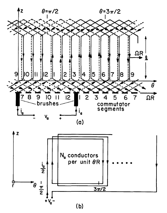
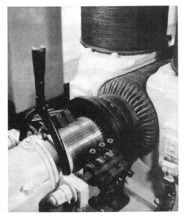
Fig.4.10.4 This venerable d-c machine,of historical interest because it generated electric power for Boston at the turn of the century, has the advantage of putting the commutator segments and brushes in clear view. The pole faces surrounding the rotor at the upper right have a shape similar to that shown in Fig.4.10.1 ,but the associated magnetic circuit is driven by armature coils wrapped on a horse-shoe magnetic circuit closing above the rotor. This is one of the first machines made after Thomas A. Edison moved from New York City to Schenectady in 1886.
Mechanical Equations
The rotor torque can be computed by integrating the Maxwell stress over a surface at \(r=R_o\) just inside the stator.This is an application of Eq.4.2.3:
\[ \tau = (2 \pi R_o l) R_o \bigg \langle B_r^F H_{\theta}^f \bigg \rangle_{\theta} \label{4} \]
Because \(\tilde{H}_{\theta m}^f = \tilde{\psi}_m^f (jm/R_o)\), and in view of the averaging theorem (Eq.2.15.17),substitution of Eqs.\ref{1} and \ref{2} converts Equation \ref{4} to
\[ \tau = 2 \pi R_o^2 l \Sigma_{m = -\infty}^{\infty} (\tilde{B}_{rm}^f)^{*} (\frac{jm}{R_o}) \tilde{\psi}_m^f \label{5} \]
With the substitution of Equation \ref{3}a into Equation \ref{5}, the "self-torque" (involving \(\tilde{\psi}_m^f (\tilde{\psi}_m^f)^{*}\)) sums to zero. (Because \(f_m/m\) is an odd function of \(m\), the mth term in the sum cancels the -mth term.) The remaining expression is a sum on \(\tilde{H}_{\theta m}^a \tilde{\psi}_m^f\). These amplitudes are evaluated using Eqs. \ref{1} and \ref{2}. The resulting magnetic torque is thus expressed as a function of the terminal currents:
\[ \tau = -G_m i_f i_a; \, G_m = \frac{16}{\pi} R R_o \ mu_o N_a n_f \Sigma_{m=1 \\ (odd)}^{+ \infty} \frac{g_m (R_o,R)}{m^2} \frac{sin (m \theta_o}{m \theta_o} \label{6} \]
The speed coefficient, \(G_m\), is positive. This is consistent with the \((\overrightarrow{J} \times \overrightarrow{B})\) density expected with \(i_f\) and \(i_s\) positive,as shown in Fig.4.10.1. But the use of the force density \(\overrightarrow{J} \times \overrightarrow{B}\) misrepresents the actual distribution of force density on the rotor.With the conductors embedded in slots of highly permeable material, the flux lines actually tend to avoid the conductors and pass through the rotor surface between the slots. This means that the magnetic flux in the region where there is a current density tends to zero as the permeability becomes infinite. In fact,the magnetic torque is largely the result of the magnetization force density acting on the rotor magnetic material between the slots. Fortunately,the stress tensor used to find Equation \ref{6} includes the magnetization force density, so the deductions are sound. But, because the stress tensor is evaluated in free space, the same calculations would be carried out and the same answer obtained even if the essential role of the magnetization force density were not recognized. That the torque is not transmitted to the rotor through the conductor is important, because it alleviates problems encountered in maintaining insulation in the face of mechanical stress and vibration.
In terms of the electrical and mechanical terminal variables \((i_f, i_a, \tau_{\theta})\), Equation \ref{6} represents the electrical-to-mechanical coupling.
Electrical Equations
To complete the model, it is necessary to express the mechanical-to-electrical coupling in terms of the terminal variables. This is done by taking advantage of Faraday's law, written for a contour of integration that is fixed in the laboratory frame of reference and passes through the appropriate winding:
\[ \oint_C (\overrightarrow{E} - \overrightarrow{v} \times \mu_o \overrightarrow{M}) \cdot d \overrightarrow{l} = - \int_S \frac{\partial{\overrightarrow{B}}}{\partial{t}} \cdot \overrightarrow{n} da \label{7} \]
For the armature, the circuit \(C\) is composed of whatever is externally connected to the terminals \((v_a,i_a)\) and the armature windings. The brushes are idealized as making continuous contact with the moving conductors. A particular possible winding that would give the uniform distribution of rotor current density is shown in Fig. 4.10.3.
The fixed frame electric field integrated on the left in Equation \ref{7} is related to the conductor current density \(\overrightarrow{J}\) by Ohm's Law, Eqs. 3.3.6, 2.5.11b, and 2.5.12b. Hence, \(\overrightarrow{E} = \overrightarrow{J}/ \sigma - \overrightarrow{v} \times \mu_o \overrightarrow{H}\) and
\[ \overrightarrow{E} - \overrightarrow{v} \times \mu_o \overrightarrow{M} = \frac{\overrightarrow{J}}{\sigma} - \overrightarrow{v} \times \overrightarrow{B} \label{8} \]
where \(\overrightarrow{v} = \Omega R \overrightarrow{i}_{\theta}\) is the velocity of the moving conductors. At a given instant, the armature winding amounts to a superimposed parallel pair of windings connected through the brushes to the armature terminals. One of the pair is shown in Fig. 4.10.3b. The other coil, represented by the dotted wires of Fig. 4.10.3a, links the same flux. Each of these windings carries half of the armature current and has the turns density \(N_a\).
For the "solid" windings, Equation \ref{7} becomes
\[v_a + \int_{wire} \frac{\overrightarrow{J}}{\sigma} \cdot d \overrightarrow{l} + \int_{wire} \Omega R B_r \overrightarrow{i}_z \cdot d \overrightarrow{l} = - \frac{d}{dt} \int_S B_r da \label{9} \]
where \(S\) is an integration over the surface enclosed by the contour \(C\) composed of the wire. The integration of \(\overrightarrow{E}\) between the terminals external to the machine gives the term \(-v_a\).
The current density in the wire is the net current \(i_a/2\) divided by the cross-sectional area of the wire, \(A_a\). Hence, the second term in Equation \ref{9} becomes
\[ \int_{wire} \frac{\overrightarrow{J}}{\sigma} \cdot d \overrightarrow{l} = \frac{i_a}{2 A_a}\frac{1}{\sigma_a} = R_a i_a; \, R_a \equiv \frac{l_a}{2 A_a \sigma_a} \label{10} \]
where \(A_a\) is the cross-sectional area of the wire and \(l_a\) is the total length of the wire joining the brushes at the given instant (the total length of the "solid" wire in Fig. 4.10.3a). Hence, \(R_a\) is the d-c resistance "seen" at the armature terminals.
The third term in Equation \ref{9} is evaluated by recognizing that those conductors between \(\theta\) and \(\theta + d \theta\) number \((N_aR)d \theta\), and therefore give a contribution \(\Omega R B_r (\theta) N_a R d \theta\). This integrand makes a positive contribution in the interval \(\pi/2 < \theta < 3 \pi/2\), where the contour is in the positive \(z\) direction, and a negative contribution in the interval \(-\pi/2 < \theta < \pi/2\) where the wires are returning in the \(-z\) direction:
\[ \int_{wire} \Omega R B_r^a \overrightarrow{i}_z \cdot d \overrightarrow{l} = l \int_{\pi/2}^{3 \pi/2} \Omega R^2 N_a B_r^a d \theta - l \int_{-\pi/2}^{\pi/2} \Omega R^2 N_a B_r^a d \theta = -4 \Omega l R^2 N_a \Sigma_{m = -\infty \\ (odd)}^{+ \infty} \frac{\tilde{B}_{rm}^a}{m} j e^{-j \frac{m \pi}{2}} \label{11} \]
The second equality results from substitution of the Fourier series and carrying out the integration.It follows from substitution for \(B_{rm}^a\) using Equation \ref{3}b with Eqs. \ref{1} and \ref{2} used to relate \(\tilde{\psi}_m^f\) and \(\tilde{H}_{\theta m}^a\) to the terminal currents that
\[ \int_{wire} \Omega R B_r^a \overrightarrow{i}_z \cdot d \overrightarrow{l} = - \Omega G_m i_f \label{12} \]
where \(G_m\) is the same as defined with Eq. \reF{6}. To complete these steps, observe that \(f_m/m^3\) is an odd function of \(m\), so that the contribution that is proportional to is sums to zero. Also, \(Rg_m(R,R_o) = -R_o g_m(R_o,R)\), as can be seen from the definition in Table 2.16.2 or by application of the reciprocity condition, Eq. 2.17.10. There is no contribution to Eg. \ref{12} of the part of \(B_r^a\) induced by the armature current because this "self-field" contribution to \(\overrightarrow{v} x \overrightarrow{B}\) at a winding location 8 is canceled by that at \(- \theta\).
To evaluate the right-hand side of Equation \ref{9}, first observe that the flux linked by the coils having their left edges in the range \(d \theta^{'}\) in the neighborhood of \(\theta^{'}\) is the product of the flux linked by one turn and the number of turns in that range of \(\theta^{'}\):
\[ - \Bigg [ l \int_{\theta^{'}}^{\theta^{'} + \pi} B_r^a R d \theta^{'} \Bigg ] N_a R d \theta^{'} \label{13} \]
As a result, the total flux linked by all of the turns is
\[ \int_S B_r da = - \int_{\pi/2}^{3 \pi/2} \Bigg [ l \int_{\theta^{'}}^{\theta^{'} + \pi} B_r^a R d \theta^{'} \Bigg ] N_a R d \theta^{'} \label{14} \]
Again, substitution of the Fourier series for \(B_r^a\) and evaluation of the integrals gives
\[ \int_S B_r da = 4 l N_a R^2 \Sigma_{m = - \infty \\ (odd)}^{ + \infty} \frac{\tilde{B}_{rm}^a}{m^2} e^{-j \frac{m \pi}{2}} \label{15} \]
Further evaluation, using Eqs. \ref{3} b, \ref{1} and \ref{2}, with the observation that gm/m3 is an odd function of \(g_m/m^3\) that the contribution proportional to if vanishes, gives
\[ \int_S B_r da = L_a i_a; \, L_a \equiv \frac{16 l N_a^2 \mu_o R^3}{\pi} \Sigma_{m=1 \\ odd}^{\infty} \frac{f_m(R_o,R)}{m^4} \label{16} \]
That \(i_f\) makes no contribution to the net flux linked by the armature winding is evident from Fig. 4.10.1.The armature and field magnetic axes are perpendicular. Thus, with the substitution of Eqs. \ref{10}, \ref{12} and \ref{16}, the armature circuit equation, Equation \ref{9}, becomes
\[ v_a = R_a i_a - \Omega G_m i_f + L_a \frac{d i_a}{dt} \label{17} \]
where \(R_a\), \(G_m\) and \(L_a\) are given by Eqs. \ref{10}, \ref{6} and \ref{16}.
The circuit equation for the field winding is similarly found by applying Faraday's integral law, Equation \ref{7}, to a contour composed of the field winding. The right-hand side of Equation \ref{7} is approximated.by the flux contribution over the surfaces of the respective poles:
\[ \int_S B_r da = n_f l \int_{-\frac{\pi}{2} + \theta_o}^{\frac{\pi}{2} - \theta_o} B_r^f R_o d \theta - n_f l \int_{\frac{\pi}{2} + \theta_o}^{\frac{3 \pi}{2} - \theta_o} B_r^f R_o d \theta \label{18} \]
Substitution of the Fourier series for \(B_r^f\) and integration gives
\[ \int_S B_r^f da = 4 n_f l R_o \Sigma_{m=1 \\ (odd)}^{\infty} \frac{e^{-j \frac{m \pi}{2}}}{(-jm)} \tilde{B}_r^f cos \, m \theta_o \label{19} \]
This expression can now be evaluated using first Equation \ref{3} a and then Eqs. \ref{1} and \ref{2}. Because \(g_m/m^3\) is an odd function of \(m\), the term proportional to \(i_a\) sums to zero with the result
\[ \int_S B_r^f da = L_f i_f ; \, L_f \equiv - \frac{16 n_f^2 l R_o \mu_o}{\pi} \Sigma_{m=1 \\ (odd)}^{\infty} \frac{cos \, m \theta_o}{m^2} \frac{sin \, m \theta_o}{m \theta_o} f_m (R,R_o) \label{20} \]

Note from the definition of \(f_m\) in Table 2.16.2 or the energy relation, Eq. 2.17.12, that \(f_m(R,R_o) < 0\),so that \(L_f\) is positive. The left-hand side of Equation \ref{7} is evaluated as for the armature except that the conductor is fixed. Hence, Equation \ref{7} becomes the required circuit equation for the field:
\[ v_f = R_f i_f + L_f \frac{d i_f}{df} \label{21} \]
The total resistance of the field winding is \(R_f = A_f l_f/ \sigma_f\), and \(L_f\) is given by Equation \ref{20}.
The Energy Conversion Process
Simple consideration of Eqs. \ref{6} and \ref{17} relates the discrete electrical and mechanical terminal variables to the energy conversion process. Consider the field excitation current if and the armature voltage va as constrained by external sources. The steady-state dependence of the armature current and the magnetic torque on the constrained variables implied by Eqs. \ref{6} and \ref{17} is then
\[ i_a = \frac{v_a}{R_a} + \frac{\Omega G_m}{R_a} i_f \label{22} \]
\[ \tau = - G_m i_f \Bigg [ \frac{v_a}{R_a} + \frac{\Omega G_m}{R_a} i_f \Bigg ] \label{23} \]
The electrical power input to the device follows from Equation \ref{22} as
\[ i_a v_a = \frac{v_a}{R_a} [v_a + \Omega G_m i_f] \label{24} \]
while the mechanical power output is given by Equation \ref{23} multiplied by the angular velocity
\[ \Omega_{\tau} = - \frac{\Omega G_m}{R_a} i_f [v_a + G_m i_f] \label{25} \]
These last two expressions are sketched in Fig. 4.10.5 to show the power-flow dependence on the field current \(i_f\) with \(\Omega\) assumed positive.
In view of the physical significance of \(i_a v_a\) and \(\Omega \tau\), it is possible to classify the regimes of operation as also sketched in Fig. 4.10.5. It is because the electromechanical coupling has been defined to include the electrical losses (by contrast with the point of view in Sec. 4.9, for example)that the brake regime is possible.
The power conversion characteristics exemplified by this d-c machine and summarized in Fig. 4.10.5are in common to the family of d-c or conduction type interactions. For example, with appropriate re-definition of variables, the same characteristics pertain to the Van de Graaff machine of Sec. 4.14.
1. H. H. Woodson and J. R. Melcher, Electromechanical Dynamics, Part I, John Wiley & Sons, New York,1968, p. 312.
2. A. E. Fitzgerald, Ch. Kingsley, Jr., and A. Kusko, Electric Machinery, McGraw-Hill Book Company,New York, 1971, p. 192.