
4.11: Green's Function Representations
- Page ID
- 43867
\( \newcommand{\vecs}[1]{\overset { \scriptstyle \rightharpoonup} {\mathbf{#1}} } \)
\( \newcommand{\vecd}[1]{\overset{-\!-\!\rightharpoonup}{\vphantom{a}\smash {#1}}} \)
\( \newcommand{\dsum}{\displaystyle\sum\limits} \)
\( \newcommand{\dint}{\displaystyle\int\limits} \)
\( \newcommand{\dlim}{\displaystyle\lim\limits} \)
\( \newcommand{\id}{\mathrm{id}}\) \( \newcommand{\Span}{\mathrm{span}}\)
( \newcommand{\kernel}{\mathrm{null}\,}\) \( \newcommand{\range}{\mathrm{range}\,}\)
\( \newcommand{\RealPart}{\mathrm{Re}}\) \( \newcommand{\ImaginaryPart}{\mathrm{Im}}\)
\( \newcommand{\Argument}{\mathrm{Arg}}\) \( \newcommand{\norm}[1]{\| #1 \|}\)
\( \newcommand{\inner}[2]{\langle #1, #2 \rangle}\)
\( \newcommand{\Span}{\mathrm{span}}\)
\( \newcommand{\id}{\mathrm{id}}\)
\( \newcommand{\Span}{\mathrm{span}}\)
\( \newcommand{\kernel}{\mathrm{null}\,}\)
\( \newcommand{\range}{\mathrm{range}\,}\)
\( \newcommand{\RealPart}{\mathrm{Re}}\)
\( \newcommand{\ImaginaryPart}{\mathrm{Im}}\)
\( \newcommand{\Argument}{\mathrm{Arg}}\)
\( \newcommand{\norm}[1]{\| #1 \|}\)
\( \newcommand{\inner}[2]{\langle #1, #2 \rangle}\)
\( \newcommand{\Span}{\mathrm{span}}\) \( \newcommand{\AA}{\unicode[.8,0]{x212B}}\)
\( \newcommand{\vectorA}[1]{\vec{#1}} % arrow\)
\( \newcommand{\vectorAt}[1]{\vec{\text{#1}}} % arrow\)
\( \newcommand{\vectorB}[1]{\overset { \scriptstyle \rightharpoonup} {\mathbf{#1}} } \)
\( \newcommand{\vectorC}[1]{\textbf{#1}} \)
\( \newcommand{\vectorD}[1]{\overrightarrow{#1}} \)
\( \newcommand{\vectorDt}[1]{\overrightarrow{\text{#1}}} \)
\( \newcommand{\vectE}[1]{\overset{-\!-\!\rightharpoonup}{\vphantom{a}\smash{\mathbf {#1}}}} \)
\( \newcommand{\vecs}[1]{\overset { \scriptstyle \rightharpoonup} {\mathbf{#1}} } \)
\(\newcommand{\longvect}{\overrightarrow}\)
\( \newcommand{\vecd}[1]{\overset{-\!-\!\rightharpoonup}{\vphantom{a}\smash {#1}}} \)
\(\newcommand{\avec}{\mathbf a}\) \(\newcommand{\bvec}{\mathbf b}\) \(\newcommand{\cvec}{\mathbf c}\) \(\newcommand{\dvec}{\mathbf d}\) \(\newcommand{\dtil}{\widetilde{\mathbf d}}\) \(\newcommand{\evec}{\mathbf e}\) \(\newcommand{\fvec}{\mathbf f}\) \(\newcommand{\nvec}{\mathbf n}\) \(\newcommand{\pvec}{\mathbf p}\) \(\newcommand{\qvec}{\mathbf q}\) \(\newcommand{\svec}{\mathbf s}\) \(\newcommand{\tvec}{\mathbf t}\) \(\newcommand{\uvec}{\mathbf u}\) \(\newcommand{\vvec}{\mathbf v}\) \(\newcommand{\wvec}{\mathbf w}\) \(\newcommand{\xvec}{\mathbf x}\) \(\newcommand{\yvec}{\mathbf y}\) \(\newcommand{\zvec}{\mathbf z}\) \(\newcommand{\rvec}{\mathbf r}\) \(\newcommand{\mvec}{\mathbf m}\) \(\newcommand{\zerovec}{\mathbf 0}\) \(\newcommand{\onevec}{\mathbf 1}\) \(\newcommand{\real}{\mathbb R}\) \(\newcommand{\twovec}[2]{\left[\begin{array}{r}#1 \\ #2 \end{array}\right]}\) \(\newcommand{\ctwovec}[2]{\left[\begin{array}{c}#1 \\ #2 \end{array}\right]}\) \(\newcommand{\threevec}[3]{\left[\begin{array}{r}#1 \\ #2 \\ #3 \end{array}\right]}\) \(\newcommand{\cthreevec}[3]{\left[\begin{array}{c}#1 \\ #2 \\ #3 \end{array}\right]}\) \(\newcommand{\fourvec}[4]{\left[\begin{array}{r}#1 \\ #2 \\ #3 \\ #4 \end{array}\right]}\) \(\newcommand{\cfourvec}[4]{\left[\begin{array}{c}#1 \\ #2 \\ #3 \\ #4 \end{array}\right]}\) \(\newcommand{\fivevec}[5]{\left[\begin{array}{r}#1 \\ #2 \\ #3 \\ #4 \\ #5 \\ \end{array}\right]}\) \(\newcommand{\cfivevec}[5]{\left[\begin{array}{c}#1 \\ #2 \\ #3 \\ #4 \\ #5 \\ \end{array}\right]}\) \(\newcommand{\mattwo}[4]{\left[\begin{array}{rr}#1 \amp #2 \\ #3 \amp #4 \\ \end{array}\right]}\) \(\newcommand{\laspan}[1]{\text{Span}\{#1\}}\) \(\newcommand{\bcal}{\cal B}\) \(\newcommand{\ccal}{\cal C}\) \(\newcommand{\scal}{\cal S}\) \(\newcommand{\wcal}{\cal W}\) \(\newcommand{\ecal}{\cal E}\) \(\newcommand{\coords}[2]{\left\{#1\right\}_{#2}}\) \(\newcommand{\gray}[1]{\color{gray}{#1}}\) \(\newcommand{\lgray}[1]{\color{lightgray}{#1}}\) \(\newcommand{\rank}{\operatorname{rank}}\) \(\newcommand{\row}{\text{Row}}\) \(\newcommand{\col}{\text{Col}}\) \(\renewcommand{\row}{\text{Row}}\) \(\newcommand{\nul}{\text{Nul}}\) \(\newcommand{\var}{\text{Var}}\) \(\newcommand{\corr}{\text{corr}}\) \(\newcommand{\len}[1]{\left|#1\right|}\) \(\newcommand{\bbar}{\overline{\bvec}}\) \(\newcommand{\bhat}{\widehat{\bvec}}\) \(\newcommand{\bperp}{\bvec^\perp}\) \(\newcommand{\xhat}{\widehat{\xvec}}\) \(\newcommand{\vhat}{\widehat{\vvec}}\) \(\newcommand{\uhat}{\widehat{\uvec}}\) \(\newcommand{\what}{\widehat{\wvec}}\) \(\newcommand{\Sighat}{\widehat{\Sigma}}\) \(\newcommand{\lt}{<}\) \(\newcommand{\gt}{>}\) \(\newcommand{\amp}{&}\) \(\definecolor{fillinmathshade}{gray}{0.9}\)In dealing with fields that are related to sources (the charge density or current density) through linear differential equations, it is possible to use yet another approach that is based on the fact that superposition of sources implies superposition of fields. This approach, which is an alternative applicable to situations illustrated in Secs. 4.5 -4.9, is familiar from the use of the superposition integral to find the potential response from charge specified throughout all space or from the Biot-Savart law for finding the magnetic field, given the distribution of current density throughout space.
Volume source distributions can often be considered the sum of distributions of surface charge or surface current. The transfer relations are a convenient vehicle for obtaining the response to such singular sources. By then integrating over the actual given source distribution, the field is represented as the sum of field responses to the surface sources.
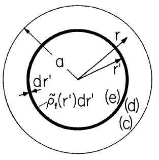
The determination of the fields and force associated with the charge beam of Sec. 4.6 illustrates the method. Figure 4.11.1 shows a cross section of the configuration pictured in Fig. 4.6.1, but with the only volume charge in a shell having radial thickness dr' at the radius r', where the density is \(\rho(r')\). The fields due to an arbitrary radial distribution of charge can be constructed once the response to this surface charge, having density \(\tilde{\rho} (r')dr'\), is determined. At the outset, consider the field to be a superposition of fields due to the potential \(\tilde{V}_o\) imposed at the surface \(r = a\) and to the distribution of charge in the volume. The latter is determined by using the boundary conditions
\[ \tilde{\phi}^c = 0, \, \tilde{\phi}^d = \tilde{\phi}^e, \tilde{D}_r^d - \tilde{D}_r^e = \tilde{\rho}(r') dr' \label{1} \]
Implicit is the understanding that there is no \(\theta\) dependence, and that the \(z\) dependence is \(exp(-jkz)\).
In the region \(r > r'\), the.flux-potential relations, Eq. (a) of Table 2.16.2, apply:
\[\begin{bmatrix} \tilde{D}^{c}_r\\ \tilde{D}^{d}_r \end{bmatrix} = \varepsilon \begin{bmatrix} f_o(r',a) & g_o(a,r') \\ g_o(r',a) & f_o(a,r') \end{bmatrix} \begin{bmatrix} \tilde{\phi}^{c}\\ \tilde{\phi}^{d} \end{bmatrix} \label{2} \]
whereas in the inner region, \(r < r'\), the limiting form of Eq. (c) is appropriate:
\[ \tilde{D}_r^e = \varepsilon f_o(0,r') \tilde{\phi}^e \label{3} \]
Subtraction of Equation \ref{3} from Equation \ref{2} b and use of the boundary conditions of Equation \ref{1} gives
\[ \tilde{\phi}^d = \tilde{\phi}^e = \frac{ \tilde{\rho}(r')dr'}{\varepsilon [ f_o(a,r') - f_o(0,r')]} \label{4} \]
By the judicious use of these amplitudes and the potential distribution given for a canonical annular region by Eq. 2.16.25, it is now possible to write the radial distribution of \(\tilde{\phi}\) for an arbitrary distribution of charge density. There are three terms. The first is simply the potential due to the voltage \(V_o\) applied at the outer wall. For this part, Eq. 2.16.25 is evaluated with \(\beta \rightarrow 0\) and \(\tilde{\phi} \alpha = \tilde{V}_o\). The second term comes from evaluating Eq. 2.16.25 for the potential at \(r\) due to the charge shell at \(r' < r\) (so that \( \alpha = a\), \(\beta = r'\), \(\tilde{\phi}^{\alpha} = \tilde{\phi}^c = 0\) and \(\tilde{\phi}^{\beta} = \tilde{\phi}^d\)) and adding up all contributions attributable to charge inside the radius of observation \(r\). Finally, the third term is written by again using Eq. 2.16.25 to express the potential, but this time due to charge at a greater radius than the \(r\), at \(r < r'\) (so that \(\alpha = r'\), \(\beta \rightarrow 0\) and \(\tilde{\phi}^{\alpha} = \tilde{\phi}^d\) and integrating over the distribution outside the observation position \(r\):
\[ \tilde{\phi} (r) = \tilde{V}_o \frac{J_o (jkr)}{J_o (jka)} + \int_o^r \frac{[J_o (jka) H_o(jkr) - H_o (jka) J_o (jkr)]}{[ J_o (jka) H_o (jkr') - H_o (jka) J_o (jkr')]} \frac{ \tilde{\rho} (r') dr'}{ \varepsilon [ f_o (a,r') - f_o (0,r')]} + \int_r^a \frac{J_o (jkr)}{J_o (jkr')} \frac{\tilde{\rho}(r') dr'}{\varepsilon [f_o(a,r') - f_o (0,r')]} \label{5} \]
To find the axial force acting on the entire beam, it is only the normal flux density at the outer wall that is required. This can be found from Equation \ref{5}, but is more easily determined directly from Eqs. \ref{2} a,used first with \(\tilde{\phi}^c = \tilde{V}_o\) and \((d) \rightarrow 0\) to find the flux density due to the wall potential alone and then with \(\tilde{\phi}^c = 0\) and \(\tilde{\phi}^d\) given by Equation \ref{4} to find the part due to the volume charge. The latter is summed over the total distribution of charge.
\[ \tilde{D}_r^c = \varepsilon f_o (0,a) \tilde{V}_o + \int_o^a \frac{ g_o (a,r') \tilde{\rho} (r') dr'}{[ f_o (a, r') - f_o (0,r')]} \label{6} \]
The force is thus determined by substituting this expression into Eq. 4.6.3. Equation \ref{6} holds for an arbitrary charge distribution, but consider the uniform distribution of charge inside the radius \(R\).Then the integration needs only be carried out from \(0\) to \(R\). With \(\tilde{V}_o\) and \(\tilde{\rho} (r')\) selected consistent with Eqs. 4.6.1 and 4.6.2, it follows that the force is given by Eq. 4.6.8 with \(L_1\) replaced by \(L_3\),where
\[ L_3 = \frac{a}{R^3} \int_o^R \frac{g_o (a,r')dr' }{[ f_o (a,r') - f_o (0,r')] } = \frac{1}{(kR)^2} \int_o^{kR} (kr') \frac{I_o (kr')}{I_o (ka)} d (kr') \label{7} \]
The integral is carried out by recognizing that \(I_o (kr')\) is a solution to Eq. 2.16.19 with \(r \rightarrow r'\) and \(m = 0\):
\[ \frac{d}{dr'} \Bigg ( r' \frac{dI_o (kr')}{dr'} \Bigg ) = k^2 r I_o (kr') \label{8} \]
Hence, Equation \ref{7} gives the same result, Eq. 4.6.13, as found in Sec. 4.6 using the "splicing approach."
The same procedure applies if the charge has 8 dependence \(exp(-jme)\). Thus, by making use of a Fourier series representation in \(\theta\) and \(z\), the method can be used to describe fields associated with arbitrary dependence on \(\theta\) and \(z\).
The Green's function approach exemplified here is applicable to modeling the synchronous machines developed in Secs. 4.7 and 4.8.\(^{1}\)
1. This is the method used by Kirtley in "Design and Construction of an Armature for an Alternator with a Superconducting Field Winding," Ph.D. Thesis, Department of Electrical Engineering, MIT,Cambridge, Mass., 1971, for a configuration closely resembling that considered in Sec. 4.8.