4.14: Van de Graaff Machine

A cross-sectional view of a Van de Graaff generator is shown in Fig. 4.14.1. An insulating belt is charged to one polarity as it passes over the lower pulley. This charge is carried upward to the essentially field-free region under the high-voltage terminal dome where it is removed and replaced by charge of opposite polarity, which then makes the return trip on the downward moving portion of the belt. Surrounding the belt are equipotential rings which help in controlling the field distribution by supporting much of the charge imaging that on the belt. The electric field consists of a generated field that is essentially vertical and a self-field associated with the charge on the belt. The equipotential rings help to insure that the self-field is essentially perpendicular to the belt surface and hence does not reinforce the generated field. To achieve relatively high electric stress (exceeding \(10^7\) V/m), the machine is operated in electronegative gases at elevated pressure.

An objective in this section, achieved while developing a lumped-parameter model for the simplified Van de Graaff generator shown in Fig. 4.14.2, is to further illustrate the use of quasi-one-dimensional models. This makes it possible to point out the analogies between d-c magnetic machines, Sec. 4.10,and what might be termed "d-c electric machines."

In several regards, the model shown in.Fig. 4.14.2 does not include features of the machine shown in Fig. 4.14.1. To avoid undue complexity, the equipotential rings are uniformly distributed between the high-voltage dome and the ground at the bottom. In the machine pictured in Fig. 4.14.1, charging is by means of a corona discharge (ion impact charging). An alternative scheme, which has the advantage of being more easily related to a physical model, makes use of induction charging of a belt consisting of conductors linked by insulators.\(^1\) For the present purposes, the belt (having thickness \(d\)) is considered to carry metallic segments that are insulated from each other. "Field" voltage sources \(v_f\) are used to induce belt charges of opposite polarity at the top and bottom. As the belt passes over the lower pulley, successive segments contact a grounded brush and hence form essentially plane-parallel capacitors having a voltage \(v_f\) across the belt thickness \(d\). With the assumption that the belt electrodes essentially cover all of the belt surface, the belt surface charge is related to the field voltage by

\[ \sigma_f = \frac{ \varepsilon v_f}{d} \label{1} \]

The current \(i_a^{i}\) both supplies the charge carried upward by the belt and neutralizes that coming downward. Hence, for a pulley angular velocity \(\Omega\) and radius \(R\),

\[ i_a^{'} = 2 \sigma_f l ( \Omega R) = \frac{2 l R \varepsilon}{d} \Omega v_f \label{2} \]

Quasi-One-Dimensional Fields

In the ideal, the generated field is uniformly distributed with respect to the z axis. To achieve this ideal, in spite of the metal pressure vessel, the equipotential rings are tapped onto a distributed bleeder resistance running from the dome to the ground plane. At least under steady-state conditions, this insures that the ring potential \(\phi_r(z)\) has the required linear distribution consistent with a uniform z-directed electric field. The following developments identify the implications of having time-varying terminal variables, \((v_a,i_a)\) and \((v_f,i_f)\).

The transverse field components are determined as though any local region along the \(z\) axis is one in which the x-directed fields are independent of \(z\). Thus, in the region between rings and pressure vessel,

\[ E_{x3} = \frac{\phi_r}{c} \label{3} \]

The fields \(E_{x2}\) and \(E_{x1}\) (Fig. 4.14.2) must satisfy Gauss' law at the belt surface and be consistent with the potential being the same on the ring where it faces the belt on the right and at the same \(z\) location on the left. Hence, with fields defined positive if they are as shown in Fig. 4.14.2,

\[ \varepsilon_o (E_{x1} + E_{x2}) = \sigma_f \label{4} \]

\[ -2 b E_{x2} + 2 a E_{x1} = 0 \label{5} \]

Here, \(E_{x2}\) is approximated as being uniform over the width of the belt, even though the rings are cylindrical and the belt is flat. The distance b is an average spacing. Simultaneous solution of these last two expressions shows that

\[ E_{x2} = \frac{\sigma_f}{\varepsilon_o (1+ \frac{b}{a})} \label{6} \]

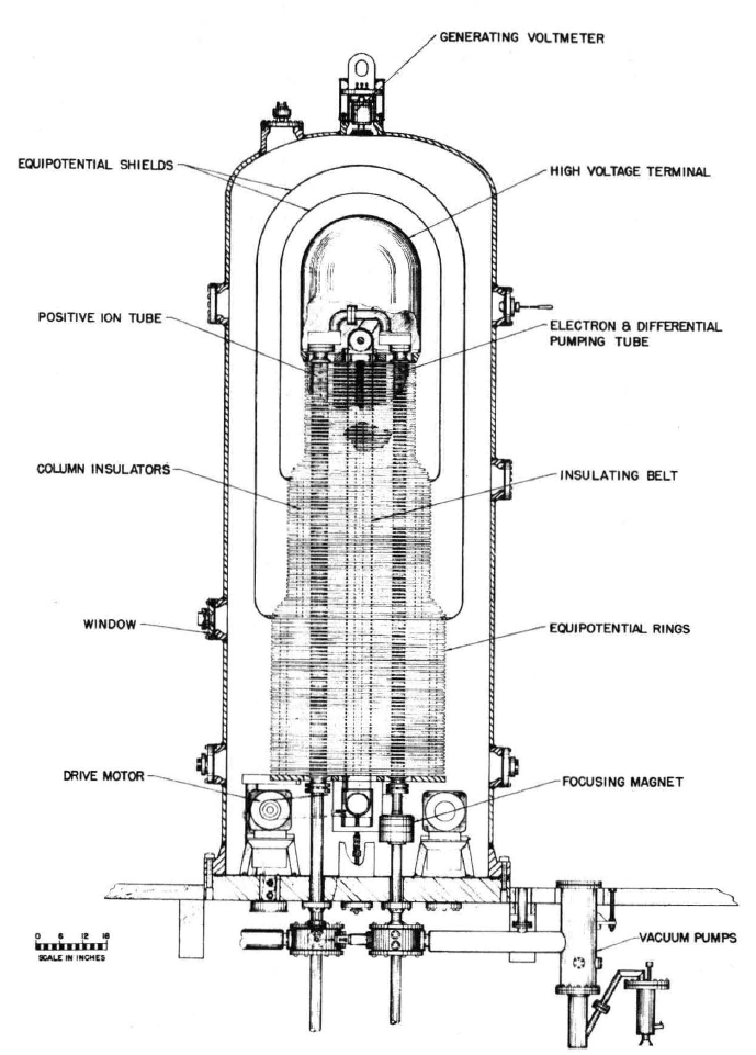
Fig.4.14.1.Cross-sectional view of Van de Graaff high-voltage generator at M.l.T., High Voltage Research Laboratory. Device, used to provide accelerator potentials in medical research, operates at terminal voltages up to 5MV.

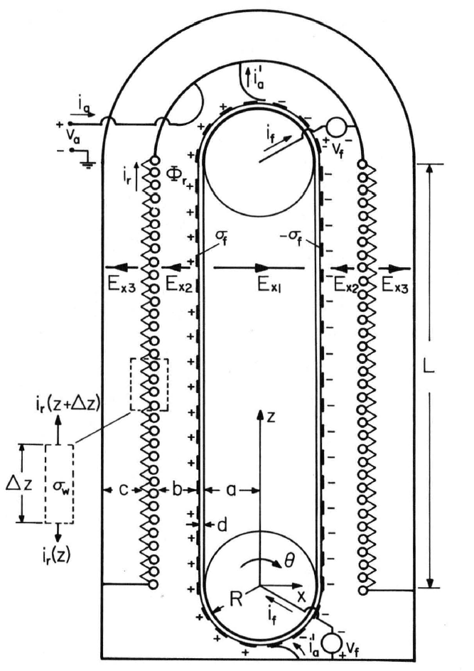
Fig.4.14.2.Model for simple Van de Graaff machine exploiting inductive charging of belt carrying metal segments.

These transverse fields make it possible to now write expressions that determine the field dependence on \(z\). A section of the ring structure having incremental length \(\Delta z\) is shown in Fig. 4.14.2. Conservation of charge for this incremental section, which takes the form of a ring-shaped volume enclosing rings in the length \(\Delta z\), is written be defining a ring charge per unit length (in the \(z\) direction), \(\lambda_r\):

\[ i_r (z + \Delta z) - i_r (z) = \frac{- \partial (\lambda_r \Delta_z)}{ \partial{t}} \label{7} \]

In the limit \(\Delta z \rightarrow 0\), Equation \ref{7} becomes

\[ \frac{\partial{i_r}}{\partial{z}} = \frac{-\partial{\lambda_r}}{\partial{t}} \label{8} \]

By symmetry, the contribution to the ring structure charge from the field inside (the images of the belt charges) cancel. What negative charge there is on the rings at the left imaging the positive belt charge on the upward-moving belt is canceled by the positive charge on the right imaging the downward moving negative belt charge. Hence, the only contribution to \(\lambda_r\) in Equation \ref{8} comes from the fields between the ring structure and the pressure vessel wall, approximated by Equation \ref{3}; \(\lambda_r \simeq 2 l \varepsilon_o \phi_r/c\). Thus, Eq. 8 becomes

\[ \frac{\partial{i_r}}{\partial{z}} = \frac{2 l \varepsilon_o}{c} \frac{-\partial{\phi_r}}{\partial{t}} \label{9} \]

A second law is required to determine the distribution of (ir,Sr). This is simply Ohm's law relating the \(z\) component of the electric field to the current carried by the bleeder resistance. With \(R_a\) the total resistance, and hence \(R_a/L\) the resistance per unit length, it follows that

\[ \frac{\partial{\phi_r}}{\partial{z}} = \frac{R_a}{L} i_r \label{10} \]

Quasistatics

There is now enough of the model developed that a meaningful discussion can be made of two quasistatic approximations implicit to a lumped parameter model for the Van de Graaff machine.

First, Equation \ref{1} is misleading in that it implies that the belt charge is instantaneously established in proportion to the field voltage over the full length of the belt. Of course, an abrupt change in \(v_f\) would result in a "wave" of surface charge carried to the high-voltage dome by the moving belt. In the model developed here, temporal variations are presumed to be long compared to a transport time \(L/ \Omega R\).With this caveat as to the dynamic range of the resulting model, the belt charge is taken as proportional to the field voltage over the full length of the machine. The machine dynamics are quasistatic relative of the time required for the belt to traverse the distance between pulleys.

A second quasistatic approximation is necessary to approximate the field distribution governed by Eqs. \ref{9} and \ref{10} in a way that leads to a lumped-parameter model. Elimination of \(i_r\) between these equations results in the diffusion equation. The potential (and hence the ring charge) diffuses in the \(z\) direction, and the resulting dynamics are not in general representable in lumped-parameter terms. The subject of charge diffusion on heterogeneous structures is taken up in Sec. 5.15. Here, the quasistatic concepts of Sec. 2.3 are revisited to obtain a low-frequency lumped parameter model. But, now the critical rate process is represented by a charge diffusion time, not an electromagnetic wave transit time.

If the fields were truly static, Equation \ref{9} shows that the current would be independent of \(z\). Thus, the zero-order current is \(i_r = i_{ro}(t)\). The associated potential distribution can then be found by integrating Equation \ref{10}:

\[ \phi_{ro} = v_a \frac{z}{L}; \, v_a = R_a i_{ro} \label{11} \]

This is the desired potential distribution. It assures a uniform generated field (z-directed) over the region of the moving belt.

Because the voltages \((v_f,v_a)\) are in general time-varying, there is an additional capacitative current. The capacitance is distributed between the high-voltage terminal and ground, and is deduced by considering the first-order current \(i_{r1}\), determined from Equation \ref{9} with the zero-order voltage (given by Equation \ref{11}) introduced for \(\phi_r\). (Note that the procedure followed here is an informal version of that outlined in Sec. 2.3.):

\[ \frac{\partial{i_{r1}}}{\partial{z}} = \frac{2 l \varepsilon_o}{c} \frac{dv_a}{dt} \frac{z}{L} \label{12} \]

The \(z\) dependence is given explicitly, so this expression can be integrated to obtain

\[ i_{r1} = \frac{l \varepsilon_o}{cL} \frac{dv_a}{dt} z^2 + f(t) \label{13} \]

with \(f(t)\) an integration function to be determined shortly by boundary conditions. Introduction of Equation \ref{13} on the right in Equation \ref{10} gives an expression for \(\phi_{r1}\) that is similarly integrated to obtain

\[ \phi_{r1} = \frac{R_a}{L} \Bigg [ \frac{l \varepsilon_o}{CL} \frac{dv_a}{da}{z^3}{3} + f(t)z \Bigg ] \label{14} \]

Because \(\phi_r = 0\) at \(z = 0\), the second integration function has been set equal to zero.

The total voltage and current distributions consist of the sum of zero and first order parts.Because the zero-order distributions already satisfy the correct boundary conditions, the first order voltage must vanish at \(z=L\). This serves to evaluate \(f(t)\) in Equation \ref{14}. If \(f(t)\) is then introduced into Equation \ref{13}, and that expression evaluated at \(z = L\), the current \(i_r(L,t)\) has been found:

\[ i_r = i_{ro} + i_{r1} = \frac{v_a}{R_a} + \frac{2 l L \varepsilon_o}{3c} \frac{dv_a}{dt} label{15} \nonumber \]

Note that because of the essentially linear distribution of voltage over the length of the structure,the equivalent capacitance is \(1/3\) what it would be if the structure formed a plane-parallel capacitor with the vessel wall. (This same equivalent capacitance can be computed with much less trouble and much less insight by simply finding the total electric energy storage and setting it equal to \(1/2 C_{eq} v_a^2)\).

Electrical Terminal Relations

The high-voltage terminal has a total current \(i_a\) which is the sum of \(-i_a\) given by Equation \ref{2}, the ring-structure current ir from Equation \ref{15}, and a current required to charge the dome. With the last of these modeled as charging half of a spherical capacitor, the high-voltage terminal relation has the form

\[ i_a = \frac{v_a}{R_a} - G_e \Omega v_f + C_a \frac{dv_a}{dt} \label{16} \]

where

\[ G_e \equiv \frac{2 l R \varepsilon}{d}; \, C-a \equiv \frac{2 l L \varepsilon_o}{3c} + 2 \pi \varepsilon_o (a+b) \nonumber \]

The field terminal relations depend on details of the specific geometry in the region of the pulleys. They take the form

\[ i_f = \frac{v_f}{R_f} + C_f \frac{dv_f}{dt} \label{17} \]

where \(R_f\) is the resistance of the belt material and the pulley mounting and \(C_f\) is the capacitance of the pulley relative to ground or to the high-voltage terminal.

Mechanical Terminal Relations

The electrical torque acting in the \(\theta\) direction on the lower pulley is computed by simply multiplying the z-directed force per unit area, \(\sigma_f E_z\), by the total belt area \(2l L\) and the lever arm \(R\). In view of Equation \ref{1} for \(\sigma_f\) and the fact that \(E_z = -v_a/L\),

\[ \tau = -G_e v_f v_a \label{18} \]

where the coefficient \(G_e\) is the same as defined with Equation \ref{16}.

Analogy to the Magnetic Machine

The terminal relations summarized by these last three equations have a canonical form not only found to describe other electric machines of quite different configuration, but also to describe magnetic d-c machines. For example, compare these relations to Eqs. 4.10.17, 4.10.21, and 4.10.6. The analogy is complete provided that the identification is \(i_f \rightarrow v_f, \, v_a \rightarrow i_a, \, R_a \rightarrow R_a^{-1}, \, G_m \rightarrow G_e\).

The Energy Conversion Process

Modes of energy conversion are explored by considering the machine constrained in such a way that the high-voltage terminal current ia is fixed, as is also the angular velocity \(\Omega\). Then, the machine is made to pass from one energy conversion regime to another by varying the field voltage \(v_f\).

Under steady-state conditions, the electrical power input is expressed by solving Equation \ref{16} for \(v_a\) and multiplying by \(i_a\):

\[ v_a i_a = R_a i_a (i_a + \Omega G_e v_f) \label{19} \]

The mechanical power output is also written in terms of \((v_f,i_a)\) by substituting for va in Equation \ref{18} and multiplying by \(\Omega\):

\[ \Omega \tau = - \Omega G_e R_a v_f (i_a + \Omega G_e v_f) \label{20} \]

With the appropriate identification of variables, plots of these expressions, and the implied modes of energy conversion, are as shown in Fig. 4.10.5.

---

1. W. D. Allen and N. G. Joyce, "Studies of Induction Charging Systems for Electrostatic Generators:The Laddertron," J. Electrostatics 1, 71-89 (1975).