
5.8: Bipolar Migration with Space Charge
- Page ID
- 51040
Charge Common conduction phenomena involve more than one charge species. Media supporting one positive and one negative species are used here to illustrate interactions between carriers caused by space-charge fields, recombination and generation. The method of characteristics is further developed as a means of understanding the evolution of the charge distributions. Based on the bipolar model of this section, the limit of ohmic conduction is examined in the next section.
Each of the charge species is governed by a conservation equation taking the form of Eq. 5.2.3:
\[ \frac{\partial{\rho_{\pm}}}{\partial{t}} + \nabla \cdot (\rho_{\pm} \overrightarrow{v} \pm \overrightarrow{J}_{\pm}^{'}) = G_{\pm} - R_{\pm} \label{1} \]
where the current density relative to the moving material is
\[ \overrightarrow{J}_{\pm}^{'} = b_{\pm} \rho_{\pm} \overrightarrow{E} \mp K_{\pm} \nabla \rho_{\pm} \label{2} \]
Consider some physical situations to which these expressions pertain. Because pairs of charged particles are generated and recombined, \(G_+ = G_{-} \equiv G\) and \(R_+ = R_{-} \equiv R\).
Positive and Negative Ions in a Gas
Perhaps by means of a corona discharge, a flame or a radio-active source, ion pairs are created and then carried into the region of interest by a gas flow or by an electric field. With the proviso that the charge per particle of each species has the same magnitude, \(q_{\pm} = q\), recombination results in the creation of a neutral particle. Carriers can recombine at a rate-that is proportional to the product of the charge densities:\(^1\)
\[ R = \frac{ \alpha \rho_{+} \rho_{-}}{q} \label{3} \]
One recombination results in the loss of one particle from each of the species,. so \(R_{\pm}\) is the same in the two equations summarized by Eq. \ref{1}.
At pressures somewhat exceeding atmospheric, the recombination coefficient a can be computed by picturing the process as one of oppositely charged particles being attracted to each other with a Coulomb force that is retarded by collisions between the ions and the neutral gas molecules. This results in the Langevin recombination coefficient:
\[ \alpha = \frac{q (b_+ + b_{-})}{\varepsilon_o} \label{4} \]
A radioactive source of \(\alpha\) or \(\beta\) particles could be used to create a generation term, \(G_{\pm}\), that would then be dependent on the density of neutral particles at not only the point in question, but points in the gas between the radioactive source and the point of interest, since these could contribute to the slowing and hence final absorption of the ionizing particle.
Aerosol Particles
Submicron particulate products of combustion are an example of macroscopic particles that often carry a natural charge of both signs. Self-agglomeration of overtly charged particles is also of interest in air pollution control.\(^2\) In these cases, the charge per particle can be many electronic charges, and so electrically induced agglomeration of oppositely charged particles does not necessarily result in a neutral particle. Rather, with the assumption that the agglomeration is stable(the particles stick), yet another species of charged particles is created and the situation is generally much more complicated than can be described by the bipolar model. But, for a mixture of uniformly charged particles, the model applies with \(G_{\pm}\) and the self-agglomeration represented by the re-combination term of Eq. \ref{3}.
Intrinsically Ionized Liquid
In liquids, thermal processes result in dissociation (ionization) of constituent molecules. For example, in pure water, a small fraction of the \(H_20\) molecules disassociate into \(H_+\) and \(OH^{-}\) ions. With these constituting the positive and negative species, there is a local thermal generation of ion pairs that is proportional to the number density, \(n\), of neutral molecules:
\[ G = \beta n \label{5} \]
and a recombination rate given by Eq. \ref{3} with \(\varepsilon_o + \varepsilon\). In the terminology of chemical kinetics, the re-combination process would be regarded as a second order rate process.\(^3\)
Partially Dissociated Salt in Solvent
When dissolved, materials such as \(NaCl\) or \(KC1\) tend to disassociate into positive and negative ions, \(Na^+C1^-\) and \(K^+Cl^-\). These then contribute to the conduction and, in this regard, can dominate over the intrinsic ionization. In that case, the conduction is represented in terms of just the two species, but it is also important to recognize that the unionized neutral molecules represent a third species. The number density, \(n\), of this species is now, like the ion number densities \(n_+\) and \(n_{-}\), a function of space and time.
To describe the evolution of the neutral particles, a conservation equation is written much as for the ions, Eq. \ref{1}. However, because these particles are not charged, the only particle current density is due to diffusion. The migration term in Eq. \ref{2} is absent. Also, generation of ion pairs now means that neutral particles are lost, and recombination means that neutrals are gained. Hence, terms on the right-hand side of the conservation equation are the negatives of those on the right in Eq. \ref{1}:
\[ \frac{\partial{n}}{\partial{t}} + \nabla \cdot (n \overrightarrow{v} - K_D \nabla n) = - \frac{G}{q} + \frac{R}{q} \label{6} \]
Summary of Governing Laws
Each of the illustrative situations that have been outlined can be described by deleting the inappropriate terms from the laws now summarized. The two charge densities contribute to Gauss' law:
\[ \nabla \cdot \varepsilon \overrightarrow{E} = \rho_+ - \rho_{-} \label{7} \]
where polarization is modeled as being linear and hence represented by the permittivity \(\varepsilon\). In the following discussions is taken as being uniform. The electric field is irrotational, and so
\[ \overrightarrow{E} = - \nabla \phi \label{8} \]
With the understanding that the given material deformations are incompressible (that \(\nabla \cdot =\overrightarrow{v} = 0\)), thecarrier evolutions are represented by Eqs. \ref{1} and \ref{2}, which in view of Gauss' law, Eq. \ref{7}, combine to become the two equations
\[ \frac{\partial{\rho_{\pm}}}{\partial{t}} + (\overrightarrow{v} \pm b_{\pm} \overrightarrow{E}) \cdot \nabla \rho_{\pm} = \mp \rho_{\pm} b_{\pm} \frac{(\rho_{+} - \rho_{-})}{\varepsilon} + \beta n - \frac{\alpha \rho_{+} \rho_{-}}{q} + K_{\pm} \nabla^2 \rho_{\pm} \label{9} \]
Here, Eqs. \ref{3} and \ref{5} are used to represent the recombination and generation. If n is a constant, or the generation term is absent, then the law governing the neutrals is not required; but if the neutral evolution is also part of the story, then Eq. \ref{6} is added to the list:
\[ \frac{\partial{n}}{\partial{t}} + \overrightarrow{v} \cdot \nabla n = - \frac{\beta n}{q} + \frac{\alpha}{q^2} \rho_{+} \rho_{-} + K_D \nabla^2 n \label{10} \]
Equations \ref{7} - \ref{10} constitute one vector and 4 scalar equations in the unknowns \(\overrightarrow{E}, \phi, \rho_{+}, \rho_{-}\) and \(n\).
Characteristic Equations
With the understanding that lengths of interest are large enough to justify ignoring the diffusion contributions to Eqs. \ref{9} and \ref{10} (typically, the ratio given by Eq. 5.2.12 is small), Eqs. \ref{9} can be written in the characteristic form introduced in Sec. 5.3:
\[ \frac{d \rho_{\pm}}{dt} = \mp \rho_{\pm} b_{\pm} \frac{ (\rho_{+} - \rho_{-}) }{\varepsilon} + \beta n - \frac{\alpha}{q} \rho_{+} \rho_{-} \label{11} \]
Here, the time rate of change is measured by an observer moving respectively with the \(\pm\) ions, on the characteristic lines
\[ \frac{d \overrightarrow{r}}{d t} = \overrightarrow{v} \pm b_{\pm} \overrightarrow{E} \label{12} \]
Similarly, Eq. \ref{10} becomes
\[ \frac{dn}{dt} = - \frac{\beta n}{q} + \frac{\alpha}{q^2} \rho_{+} \rho_{-} \label{13} \]
on the characteristic lines that are physically the particle lines for the neutrals
\[ \frac{d \overrightarrow{r}}{d t} = \overrightarrow{v} \label{14} \]
Following a particle of the neutral material, the neutral number density changes with time inaccordance with the local balance between generation and recombination. What makes the bipolar situation more complex than for unipolar migration is that not only are the positive and negative species described by Eqs. \ref{11} along different characteristic lines, but the space-charge term on the right has an effect that is proportional to the net charge, generally with contributions from both species.
One-Dimensional Characteristic Equations
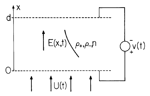
Consider the one-dimensional configuration, illustrated by Fig. 5.8.1, in which densities and fields are independent of \((y,z)\), with \(\overrightarrow{E} = E(x,t) \overrightarrow{i}_x\) and \(overrightarrow{v} = U(t) \overrightarrow{i}_x\) .Because \(\overrightarrow{v}\) is solenoidal, \(U\) is at most a function of time only. Then, Eqs. \ref{11} - \ref{14} reduce to the first six ordinary differential equations summarized by Eq. \ref{15}:
\[ \frac{d}{dt} \begin{bmatrix} \rho_+ \\ \rho_{-} \\ x_+ \\ x_{-} \\ n \\ x_n \\ E_+ \\ E_{-} \\ E_n \end{bmatrix} = \begin{bmatrix} - \frac{b_+}{\varepsilon} \rho_+ (\rho_+ - \rho_{-} ) + \beta n - \frac{\alpha}{q} \rho_{+} \rho_{-} \\ \frac{b_{-}}{\varepsilon} \rho_{-} (\rho_+ - \rho_{-} ) + \beta n - \frac{\alpha}{q} \rho_{+} \rho_{-} \\ U + b_+ E_+ \\ U - b_{-} E_{-} \\ - \frac{\beta}{q} n + \frac{\alpha}{q^2} \rho_+ \rho_{-} \\ U \\ - \frac{(b_+ + b_{-})}{\varepsilon} \rho_{-} E_+ + \frac{C(t)}{\varepsilon} \\ - \frac{(b_+ + b_{-})}{\varepsilon} \rho_{+} E_{-} + \frac{C(t)}{\varepsilon} \\ - \frac{1}{\varepsilon} (b_+ \rho_+ + b_{-} \rho_{-}) E_n + \frac{C(t)}{\varepsilon} \end{bmatrix} \label{15} \]
where
\[ \frac{C(t)}{\varepsilon} \equiv \frac{1}{d} \Big \{ \frac{dv}{dt} + \frac{1}{\varepsilon} \int_0^d [ \rho_+ (U + b_+ E) - \rho_{-} (U - b_{-} E)] dx \Big \} \nonumber \nonumber \]
Here, subscripts are used to distinguish the characteristic lines. Thus the first two equations respectively apply along lines in the \((x-t)\) plane represented respectively by the third and fourth expressions. Similarly, the fifth equation applies along the lines defined by the sixth expression.
In numerically integrating these equations it is convenient to take account of Gauss' law, Eq. \ref{7},by having equations for the time rates of change of the electric field for an observer moving along of the respective characteristic lines.\(^4\) each To this end, the time rate of change of Eq. \ref{7} is written as
\[ \frac{\partial}{\partial{x}} (\frac{\partial{E}}{\partial{t}}) = \frac{1}{\varepsilon} \frac{\partial}{\partial{t}} (\rho_+ - \rho_{-}) \label{16} \]
The difference between Eqs. \ref{9} becomes
\[ \frac{\partial}{\partial{t}} (\rho_+ - \rho_{-}) + \frac{\partial}{\partial{x}} [ \rho_+ (U + b_+ E) - \rho_{-} (U - b_{-} E)] = 0 \label{17} \]
Elimination of the term in \(\rho_{+} - \rho_{-} \) between these equations leads to the conclusion that
\[ \frac{\partial}{\partial{x}} \Big [ \varepsilon \frac{\partial{E}}{\partial{t}} + [ \rho_+ (U + b_{+} E) - \rho_{-} (U - b_E)] \Big ] = 0 \label{18} \]
The quantity in brackets, the sum of the displacement current and the migration currents, is defined as \(C(t)\). Integration of \(C(t)\) from \(x = 0\) to \(x = d\) results in the expression given with Eq. \ref{15}. The voltage \ref{v}, defined as the integral of \(E\) between the planes \(x = 0\) and \(x = l\), brings in the remaining field law, Eq. \ref{8}.
Gauss' law can be used to eliminate the net charge \(\rho_{+} - \rho_{-} \) from \(C(t)\), the quantity in brackets in Eq. \ref{18}, to obtain
\[ \frac{\partial{E}}{\partial{t}} + U \frac{\partial{E}}{\partial{x}} = \frac{C(t)}{\varepsilon} - \frac{1}{\varepsilon} (b_+ \rho_{+} - b_{-} \rho_{-}) E \label{19} \]
What is on the left is the time rate of change of \(E\) for an observer moving on the neutral characteristic lines. Thus, Eq. \ref{19} is the last of Eqs. \ref{15}. To obtain the time rates of change of \(E\) on the charged particle characteristic lines, add to both sides of Eq. \ref{19} \(\pm b_{\pm} E \partial{E} / \partial{x}\). On the left is then the time rate of change of \(E\) for an observer moving on the respective characteristic lines \(x_{\pm}\). With Gauss' law used to replace \(\partial{E} / \partial{x}\) on the right with \((\rho_{+} - \rho_{-})/ \varepsilon\), these equations become the seventh and eighth expressions of Eq. \ref{15}.
The functions \(E_+(t), E_{-}(t)\) and \(E_n(t)\) are numerically the same as \(E(x,t)\). Each is now regarded as solely a function of time because it is understood that the respective functions are measured by an observer moving along the lines \(x_+(t), x_{-} (t)\), and \(x_n(t)\), respectively.
Numerical Solution
A beauty of the method of characteristics is that it reduces partial differential equations to a system of ordinary differential equations, Eqs. \ref{15}. Many numerical techniques exist for integrating nonlinear equations in this form, e.g., Runge-Kutta or predictor-corrector.\(^5\)
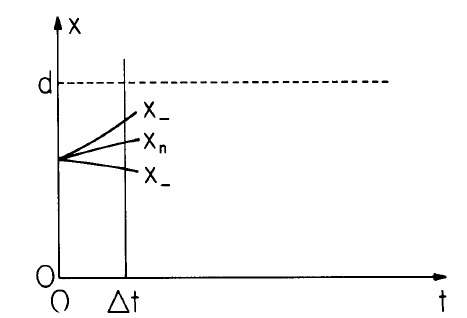
The region of interest in the \((x-t)\) plane is bounded by \(x = 0\) and \(x = d\), where screen electrodes are respectively constrained to potential \(v(t)\) and \(0\). These planes define two sides of a \("U"\) shapedregion, sketched in Fig. 5.8.2, with the initial line \(t = 0\) the third side. Wherever one of the characteristic lines \((x_+, x_{-}, x_n)\) enters this region, there must be a condition on the associated density \(\rho_+, \rho_{-}\) or \(n\). In addition, the potential of the boundaries at \(x = 0\) and \(x = d\) is constrained. Thus, when \(t = 0\), characteristic lines enter the region with the initial values of \(\rho_+, \rho_{-}\) and \(n\). Taken with the constraint on the potential difference between the screens, this determines the initial distribution of \(E(x,0)\), because at any time, Gauss' law can be integrated to obtain
\[ E(x) = \int_0^x \frac{(\rho_+ - \rho_{-})}{\varepsilon} dx^{'} + E_o \label{20} \]
The constant of integration, \(E_o\) , is determined by integrating \(E\) from \(x = 0 \) to \(x = d\) and requiring that the result be \(v\). If the resulting value of \(E_o\) is substituted back into Eq. \ref{20}, an expression is obtained for \(E(x,t)\) in terms of \(\rho_+\) and \(\rho_{-}\) when \(t = t\):
\[ E(x,t) = \int_0^x \frac{(\rho_+ - \rho_{-})}{\varepsilon} dx^{'} - \frac{1}{d} \int_0^d dx \int_0^x \frac{(\rho_+ - \rho_{-})}{\varepsilon} dx^{'} + \frac{v}{d} \label{21} \]
With the initial values of all quantities on the right in Eq. \ref{15} established, it is now possible to begin marching forward in time.
In the integration scheme used to generate the distributions shown, a predictor-corrector sub-routine is used which calls a user-written subroutine for evaluation of derivatives (Eqs. \ref{15}) after each prediction or correction step. Because Eqs. \ref{15} are a set of coupled ordinary nonlinear differential equations, there are readily available routines for carrying out the main integration (compiled subroutines for predictor-corrector integration are available, for example, in the International Mathematical & Statistical Library).
Note that the derivatives are not entirely determined by quantities naturally evaluated on the same characteristic line. For example, \(d \rho_+/dt\) is determined by not only \(\rho_+\), but by \(\rho_{-}\) and \(n\) as well,and these quantities are naturally found along their respective characteristic lines. If the distanced is broken into \((i -1)\) segments, there are (i) characteristic lines of each family emanating from the t=0 line into the region of interest. Equations \ref{15} comprise (\ref{9} i) coupled ordinary differential equations. The equations for values on a (+) characteristic line are coupled to those on neighboring characteristic lines by Eqs. \ref{15} b and \ref{15} e, and coupled to all the other characteristic lines thru \(C(t)\).Thus, at each step in time, values of \(\rho_{-}\) and \(n\) on the \(x_+\) characteristic must be interpolated from values on the neighboring characteristics \(x_{-}\) and \(x_n\). Similarly, values of \(\rho_+\) and \(n\) must be interpolated from their respective characteristic lines onto the \(x_{-}\) lines for use in the equation for \(\rho_{-}\),and values of \(\rho_+\) and \(\rho_{-}\) must be interpolated onto the neutral characteristics in order to compute \(dn/dt\). The interpolation for the examples illustrated here are done with a four-point Lagrangian formula. This fits a cubic equation to the nearest two data points on both sides of the interpolation point.
The charge and neutral density profiles are conveniently initiated with step singularities. In order to prevent the smearing out of these step edges, a two-point (linear) interpolation is used when near these edges, so that the data on one side of the edge does not influence the interpolated values on the other side.
The integration in \(C(t)\) is carried out in two parts: the \(\rho_+ (U_+ + b_+E)\) term is integrated over the (irregular) set of \(x_+\) points using the readily available values of \(\rho_+\) and \(E_+\) on these points, and the \(\rho_{-} (U - b_{-} E)\) term is similarly integrated over the \(x_{-}\) points.
Numerical Example
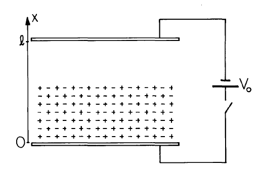
(The numerical analysis of this section was carried out by R. S. Withers)A situation which is the basis for gaining physical insights in this and the next section is sketched in Fig. 5.8.3. When \(t = 0\), equal amounts of positive and negative charge uniformly occupy the region next to the lower screen, with the region above initially free of charge. Initially, neutral particles are absent throughout and there is no generation at any time. Because the effect of the convection in one dimension is to translate the material in the x direction, the material velocity \(U\) is taken as zero. Hence, the model is appropriate to describing what might be considered a "conducting layer" adjacent to an insulating layer of material sandwiched between plane-parallel electrodes. It is assumed that charged particles leaving the region by arriving at one or the other of the electrodes are neutralized and removed from the volume. Further, charged particles cannot be generated at the electrode surfaces, and hence characteristic lines emanating from the electrodes carry no associated particle density.
The evolution of electric field and net charge are displayed in Fig. 5.8.4a, where the \(x-t\) plane forms the "floor." Similarly, the \(x-t\) dependence of the particle densities is shown in Fig. 5.8.4b.The critical characteristic lines, \(x_+\) and \(x_{-}\), are also shown in these plots. (The neutral characteristics, \(x_n\), are simply lines running parallel to the \(t\) axis.)
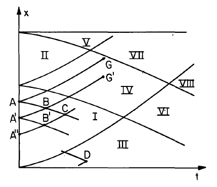
Considerable insight can be extracted from this example by identifying the dominant processes in each of the regions demarked in Fig. 5.8.5 by critical characteristic lines. In region \(I\), bounded by \(x_+\) originating at the lower electrode and x. originating at the initial interface between the charged layer and the region above, the initial charge densities at \(A\), \(A'\), and \(A"\) are the same. It follows that these initial points can be chosen such that \(B\) and \(B'\) occur at the same time (on the same line \(t = constant\)). Also, the initial conditions are the same so the values of \(\rho_+\) and of \(\rho_{-}\). at the points \(B\) and \(B'\) are the same. In turn, the value of the charge densities at \(C\) are the same as at other positions in region \(I\) at this same time. It is concluded that Eqs. \ref{15}a and \ref{15}b describe the time dependence at any given fixed location \(x\) in region \(I\). In the example, initial conditions set \(\rho_+ = \rho_{-}\) and these equations reduce to the same equation for subsequent times. Thus, the net charge density \(\rho_+ - \rho_{-}\) is zero in region \(I\), and, through recombination alone, the individual charge species decay ac-cording to the law
\[ \rho_+ = \frac{\rho_o}{1 + t/\tau} \, \tau = \frac{\varepsilon_o}{\rho_o (b_+ + b_{-})} \label{22} \]
where Eq. 5.8.4, the Langevin recombination coefficient, has been used.
Because there is no generation, the recombination simply feeds the neutral equation, and Eq. \ref{15} e shows that in region \(I\)
\[ n = \int_0^t \frac{\rho_o}{q} \frac{d(t^{'}/\tau)}{(1+t^{'}/ \tau)^2} = \frac{\rho_o}{q} \frac{t/\tau}{(1+ t/\tau)} \label{23} \]
Region \(II\), like region \(I\), has uniform initial conditions, so the same arguments apply. But, the initial conditions on \((\rho_+, \rho_{-},n)\) are all zero, and so these quantities remain zero throughout. It follows from the characteristic electric field equations, Eqs. \ref{15}g - \ref{15}j, that \(E\) is uniform in this region.
In region \(III\), the \(x_+\) characteristics enter from the lower electrode carrying no \(\rho_+\). At a point like \(D\), Eq. \ref{15} a establishes \(\rho_+ = 0\), and a step-by-step march into this region shows that at each point \(\rho_+ = 0\). Hence, Eq. \ref{15} b applies with \(\rho_+ = 0\) and it is concluded that along \(x\). in this region the charge evolution is as though the process were the unipolar self-precipitation process discussed in Sec. 5.6. Because there are only negative charges, there is no recombination.
Region \(IV\), where the positive charges are moving upward along the \(E\) lines but the negative charges have been swept downward, is of essentially the unipolar character of region \(III\). Because charges do not originate on the upper electrode, region \(VII\) is also unipolar.
Finally, it can be argued that in regions \(V, VI\) and \(VIII\), \(\rho_+ = 0\) and \(\rho_{-} = 0\).
The neutral characteristics, xn, do not enter into the classification of regimes because the coupling to \(n\) is "one-way." But, neutrals created by recombination remain behind the \(x\). wavefront defining the demarcation of regions \(IV\) and \(I\). As a result, the distribution of \(n\) at a given time is uniform in region \(I\) (with amplitude given by Eq. \ref{23}) and makes a smooth transition to zero at the initial location of the region \(IV-I\) interface.
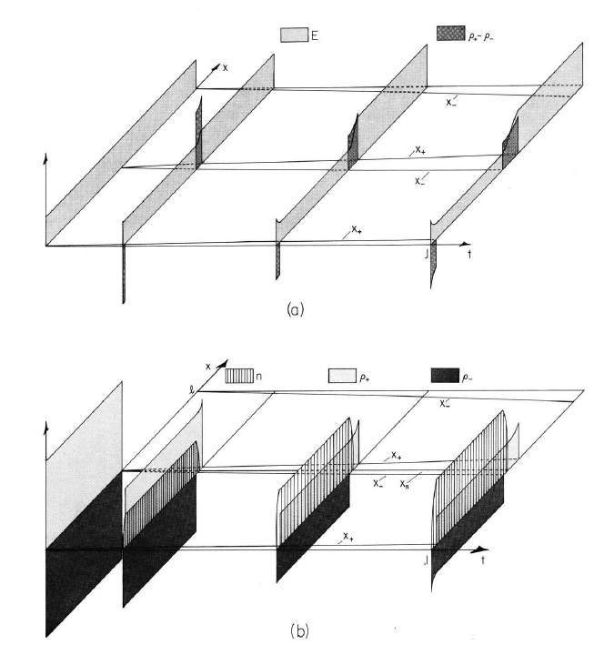
Fig.5.8.4. Evolution of layer composed of equal densities of positive and negative carrier so ccupying lower half of region between capacitor plates. Initially there are no neutrals. Generation is absent \((\beta=0)\) so recombination results in neutrals. For the case shown, \(t= \underline{t} [ l/\xi (b_+ + b_{-})]\), ,where \(\xi = V_o/l\). Also, \(b_+ = b_{-}\) and the initial charge densities are such that \(\rho_+ = \rho_{-} = 30 (\varepsilon V_o/l^2)\). (a) Electric field and net charge density;(b) neutral density and positive and negative charge densities.
At a given instant, the net charge in region \(IV\) increases with \(x\). The reason for this is apparent from following the \(x_+\) characteristic originating at \(A\) in Fig. 5.8.5. At first, \(\rho_+\) decays by recombination, with a time constant \(\tau = \varepsilon_o / \rho_o (b_+ + b_{-})\), until \(x_+\) passes from regime \(I\) to region \(IV\). The subsequent decay is due to self-precipitation and occurs with the larger (slower) unipolar time constant \(\varepsilon_o / \rho_o b_+\). Thus, at \(G\) in Fig. 5.8.5, particles have spent more time in the unipolar regime and less time in the recombination regime than those at \(G'\). This is.why, at a given instant in Fig. 5.8.4a, the net charge at the \(x_+\) wavefront of the regime \(IV\) (which is decaying at the unipolar rate) is greater than behind the front. (Note,however, that the po used in evaluating this latter time constant is the value of \(\rho_+\) when the characteristic line enters region \(IV\), which is not the same for points \(G\) and \(G'\).
1. S. C. Brown, "Conduction of Electricity in Gases," in Handbook of Physics, E. U. Condon and H. Odishaw, eds., McGraw-Hill Book Company, New York, Toronto, London, 1958, pp. 4-166.
2. J. R. Melcher, K. S. Sachar and E. P. Warren, "Overview of Electrostatic Devices for Control of Submicrometer Particles," Proc. IEEE 65, 1659 (1977).
3. K. J. Laidler, Chemical Kinetics, McGraw-Hill Book Company, New York, 1965, p. 535.
4. M. Zahn, "Transient Electric Field and Space Charge Behavior for Drift Dominated Bipolar Conduction,"in Conduction and Breakdown in Dielectric Liquids, J. M. Goldschvartz, ed., Delft University Press,1975, pp. 61-64.
5. F. S. Acton, Numerical Methods that Work, Harper & Row, Publishers, New York, 1970.