1.4: Review of laser Essentials

Linear and ring cavities:

Figure 1.9: Possible cavity configurations. (a) Schematic of a linear cavity laser. (b) Schematic of a ring laser. [1]

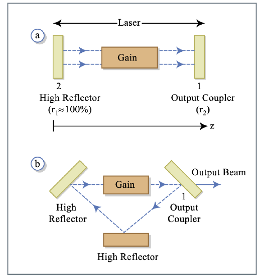
Steady-state operation: Electric field must repeat itself after one roundtrip. Consider a monochromatic, linearly polarized field

\[E(z, t) = \Re\{ E_0 e^{j(\omega t - kz)}\}, \nonumber \]

where

\[k = \dfrac{\omega}{c} n \nonumber \]

is the propagation constant in a medium with refractive index \(n\).

Consider linear resonator in Figure 1.9a. Propagation from (1) to (2) is determined by \(n = n' + jn''\) (complex refractive index), with the electric field given by

\[E = \Re \{ E_0 e^{\tfrac{\omega}{c} n_g'' \ell_g} e^{j\omega t} e^{-j \tfrac{\omega}{c}(n_g' \ell_g + \ell_a)} \}, \nonumber \]

where \(n_g\) is the complex refractive index of the gain medium (outside the gain medium \(n = 1\) is assumed), \(\ell_g\) is the length of the gain medium, \(\ell_a\) is the outside gain medium, and \(\ell = n_g \ell_g + \ell_a\) is the optical path length in the resonator.

Propagation back to (1), i.e. one full roundtrip results in

\[E = \Re \{ r_1 r_2 e^{2\tfrac{\omega}{c} n_g'' \ell_g} E_0 e^{j\omega t -j 2 \tfrac{\omega}{c} \ell} \} \Rightarrow r_1 r_2 e^{2 \tfrac{\omega}{c} n_g'' \ell_g} = 1, \nonumber \]

i.e. the gain equals the loss, and furthermore, we obtain the phase condition

\[\dfrac{2\omega \ell}{c} = 2m\pi. \nonumber \]

The phase condition determines the resonance frequencies, i.e.

\[\omega_m = \dfrac{m\pi c}{\ell} \nonumber \]

and

\[f_m = \dfrac{mc}{2\ell}. \nonumber \]

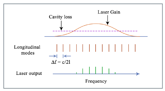
The mode spacing of the longitudinal modes is

\[\Delta f = f_m - f_{m - 1} = \dfrac{c}{2\ell} \nonumber \]

(only true if there is no dispersion, i.e. \(n \ne n(\omega)\)). Assume frequency independent cavity loss and bell shaped gain (see Figure 1.10).

Figure 1.10: Laser gain and cavity loss spectra, longitudinal mode location, and laser output for multimode laser operation.

Figure 1.11: Gain and loss spectra, longitudinal mode locations, and laser output for single mode laser operation.

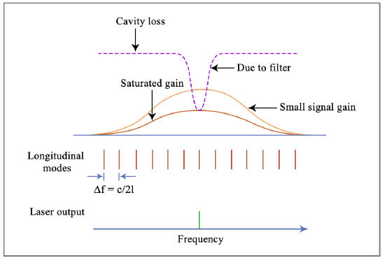
To assure single frequency operation use filter (etalon); distinguish be- tween homogeneously and inhomogeneously broadened gain media, effects of spectral hole burning! Distinguish between small signal gain g0 per roundtrip, i.e. gain for laser intensity \(I \to 0\), and large signal gain, most often given by

\[g = \dfrac{g_0}{1 + \tfrac{I}{I_{sat}}}, \nonumber \]

where \(I_{sat}\) is the saturation intensity. Gain saturation is responsible for the steady state gain (see Figure 1.11), and homogeneously broadened gain is assumed.

To generate short pulses, i.e. shorter than the cavity roundtrip time, we wish to have many longitudinal modes runing in steady state. For a multimode laser the laser field is given by

\[E(z, t) = \Re \left [ \sum_{m} \hat{E}_m e^{j(\omega_m t - k_m z + \phi_m)} \right ], \nonumber \]

\[\omega_m = \omega_0 + m \Delta \omega = \omega_0 + \dfrac{m\pi c}{\ell}, \nonumber \]

\[k_m = \dfrac{\omega_m}{c}, \nonumber \]

where the symbol \(\hat{\ }\) denotesa frequency domain quantity. Equation (1.4.10) can be rewritten as

\[E(z,t) = \Re \left \{e^{j \omega_0 (t - z/c) \sum_m \hat{E}_m e^{j (m \Delta \omega (t - z/c) + \phi_m)} \right\} \nonumber \]

\[= \Re [A(t - z/c) e^{j\omega_0 (t - z/c)} ] \nonumber \]

with the complex envelope

\[A(t - \dfrac{z}{c}) = \sum_m E_m e^{j (m \Delta \omega (t - z/c) + \phi_m)} = \text{complex envelope (slowly varying).} \nonumber \]

\(e^{j\omega_0 (t - z/c)\) is the carrier wave (fast oscillation). Both carrier and envelope travel with the same speed (no dispersion assumed). The envelope function is periodic with period

\[T = \dfrac{2\pi}{\Delta \omega} = \dfrac{2\ell}{c} = \dfrac{L}{c}. \nonumber \]

\(L\) is the roundtrip length (optical)!

Example \(\PageIndex{1}\)

We assume \(N\) modes with equal amplitudes \(E_m = E_0\) and equal phases \(\phi_m = 0\), and thus the envelope is given by

\[A (z, t) = E_0 \sum_{m = -(N-1)/2}^{(N - 1)/2} e^{j(m \Delta \omega (t - z/c))} \nonumber \]

With

\[\sum_{m = 0}^{q - 1} a^m = \dfrac{1 - a^q}{1 - a}, \nonumber \]

we obtain

\[A(z, t) = E_0 \dfrac{\sin [\tfrac{N \Delta \omega}{2} ( t - \tfrac{z}{c})]}{\sin [\tfrac{\Delta \omega}{2} ( t - \tfrac{z}{c})]} \nonumber \]

The laser intensity \(I\) is proportional to \(E(z,t)^2\), averaged over one optical cycle: \(I \sim |A(z, t)|^2\). At \(z = 0\), we obtain

\[I(t) \sim |E_0|^2 \dfrac{\sin^2 (\tfrac{N \Delta \omega t}{2})}{\sin^2 (\tfrac{\Delta \omega t}{2})}. \nonumber \]

Figure 1.12: (a) mode-locked laser output with constant mode phase. (b) Laser output with randomly phased modes.

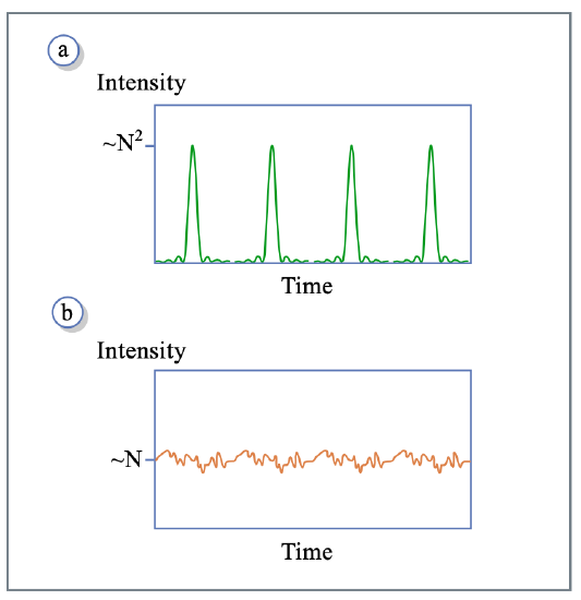
(a) Periodic pulses given by Equation 1.4.19, period \(T = 1/ \Delta f = L/c\)

• pulse duration

\[\Delta t = \dfrac{2\pi}{N \Delta \omega} = \dfrac{1}{N\Delta f} \nonumber \]

• peak intensity ~ \(N^2 |E_0|^2\)
• average intensity ~ \(N |E_0|^2 \Rightarrow\) peak intensity is enhanced by a factor \(N\).

(b) If phases of modes are not locked, i.e. \(\phi_m\) random sequence

• Intensity fluctuates randomly about average value (\(\sim N |E_0|^2\)), same as modelocked case

• correlation time is \(\Delta t_c \approx \dfrac{1}{N \cdot \Delta f}\)

• Fluctuations are still periodic with period \(T = 1/\Delta f\).

In a usual multimode laser, \(\phi_m\) varies over \(t\).