5.2: Active Mode Locking by Loss Modulation

Active mode locking was first investigated in 1970 by Kuizenga and Siegman using a gaussian pulse analyses, which we want to delegate to the exercises [3]. Later in 1975 Haus [4] introduced the master equation approach (5.1.21). We follow the approach of Haus, because it also shows the stability of the solution.

Image removed due to copyright restrictions. Please see: Keller, U., Ultrafast Laser Physics, Institute of Quantum Electronics, Swiss Federal Institute of Technology, ETH Hönggerberg—HPT, CH-8093 Zurich, Switzerland.

Figure 5.3: Schematic representation of the master equation for an actively mode-locked laser.

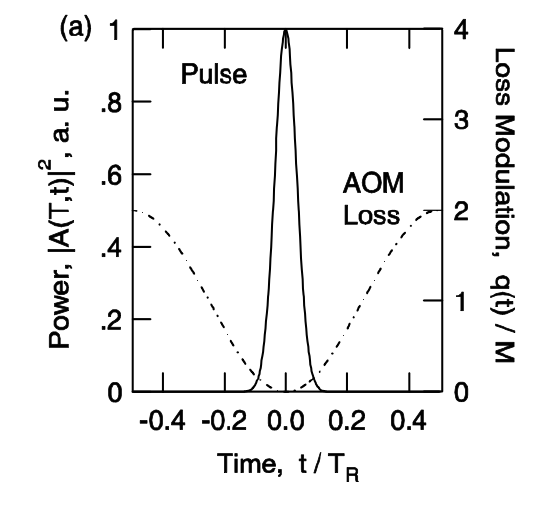
We introduce a loss modulator into the cavity, for example an acousto-optic modulator, which periodically varias the intracavity loss according to \(q(t) = M(1- \cos (\omega_M t))\). The modulation frequency has to be very precisely tuned to the resonator round-trip time, \(\omega_M = 2 \pi /T_R\), see Figure 5.2. The modelocking process is then described by the master equation

\[T_R \dfrac{\partial A}{\partial T} = \left [g(T) + D_g \dfrac{\partial^2}{\partial t^2} - l - M (1 - \cos (\omega_M t)) \right ] A.\label{eq5.2.1} \]

neglecting GDD and SPM. The equation can be interpreted as the total pulse shaping due to gain, loss and modulator, see Fig.5.3.

If we fix the gain in Equation (\(\ref{eq5.2.1}\)) at its stationary value, what ever it might be, Equation (\(\ref{eq5.2.1}\)) is a linear p.d.e, which can be solved by separation of variables. The pulses, we expect, will have a width much shorter than the round-trip time TR. They will be located in the minimum of the loss modulation where the cosine-function can be approximated by a parabola and we obtain

\[T_R \dfrac{\partial A}{\partial T} = \left [g - l + D_g \dfrac{\partial^2}{\partial t^2} - M_s t^2 \right ]A.\label{eq5.2.2} \]

\(M_s\) is the modulation strength, and corresponds to the curvature of the loss modulation in the time domain at the minimum loss point

\[D_g = \dfrac{g}{\Omega_g^2}, \nonumber \]

\[M_s = \dfrac{M \omega_M^2}{2}. \nonumber \]

The differential operator on the right side of (\(\ref{eq5.2.2}\)) corresponds to the Schrödinger-Operator of the harmonic oscillator problem. Therefore, the eigen functions of this operator are the Hermite-Gaussians

\[A_n (T, t) = A_n (t) e^{\lambda_n T/ T_R},\label{eq5.2.5} \]

\[A_n (t) = \sqrt{\dfrac{W_n}{2^n \sqrt{\pi} n! \tau_a}} H_n (t/ \tau_a) e^{-\tfrac{t^2}{2\tau_a^2}}, \nonumber \]

where \(\tau_a\) defines the width of the Gaussian. The width is given by the fourth root of the ratio between gain dispersion and modulator strength

\[\tau_a = \sqrt[4]{D_g/M_s}.\label{eq5.2.7} \]

Note, from Equation (\(\ref{eq5.2.5}\)) we can follow, that the gain per round-trip of each eigenmode is given by \(\lambda_n\) (or in general the real part of \(\lambda_n\)), which are given by

\[\lambda_n = g_n - l - 2M_s \tau_a^2 (n + \dfrac{1}{2}).\label{eq5.2.8} \]

The corresponding saturated gain for each eigen solution is given by

\[g_n = \dfrac{1}{1 + \tfrac{W_n}{P_L T_R}}, \nonumber \]

where Wn is the energy of the corresponding solution and \(P_L = E_L/\tau_L\) the saturation power of the gain. Equation (\(\ref{eq5.2.8}\)) shows that for given \(g\) the eigen solution with \(n = 0\), the ground mode, has the largest gain per roundtrip. Thus, if there is initially a field distribution which is a superpostion of all eigen solutions, the ground mode will grow fastest and will saturate the gain to a value

\[g_s = l + M_s \tau_a^2.\label{eq5.2.10} \]

such that \(\lambda_0 = 0\) and consequently all other modes will decay since \(\lambda_n < 0\) for \(n \ge 1\). This also proves the stability of the ground mode solution [4]. Thus active modelocking without detuning between resonator round-trip time and modulator period leads to Gaussian steady state pulses with a FWHM pulse width

\[\Delta t_{FWHM} = 2 \ln 2 \tau_a = 1.66 \tau_a. \nonumber \]

The spectrum of the Gaussian pulse is given by

\[\tilde{A}_0 (\omega) = \int_{-\infty}^{\infty} A_0 (t) e^{i \omega t} dt \nonumber \]

\[= \sqrt{\sqrt{\pi} W_n \tau_a} e^{-\tfrac{(\omega \tau_a)^2}{2}}, \nonumber \]

and its FWHM is

\[\Delta f_{FWHM} = \dfrac{1.66}{2\pi \tau_a}. \nonumber \]

Therfore, the time-bandwidth product of the Gaussian is

\[\Delta t_{FWHM} \cdot \Delta f_{FWHM} = 0.44. \nonumber \]

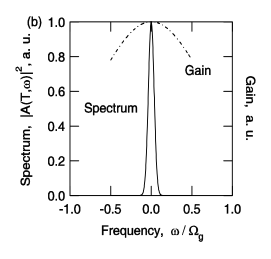
The stationary pulse shape of the modelocked laser is due to the parabolic loss modulation (pulse shortening) in the time domain and the parabolic filtering (pulse stretching) due to the gain in the frequency domain, see Figs. 5.4 and 5.5. The stationary pulse is achieved when both effects balance. Since external modulation is limited to electronic speed and the pulse width does only scale with the inverse square root of the gain bandwidth actively modelocking typically only results in pulse width in the range of 10-100ps.

Figure 5.4: (a) Loss modulation gives pulse shortening in each roundtrip

Figure 5.5: (b) the finite gain bandwidth gives pulse broadening in each roundtrip. For a certain pulse width there is balance between the two processes.

For example: \(\ce{Nd: YAG}\); \(2l = 2g = 10%\), \(\Omega_g = \pi \Delta f_{FWHM} = 0.65\) THz, \(M = 0.2\), \(f_m = 100\) MHz, \(D_g = 0.24 \ \text{ps}^2\), \(M_s = 4 \cdot 10^{16} s^{-1}\), \(\tau_p \approx 99 \ \text{ps}\).

With the pulse width (\(\ref{eq5.2.7}\)), Eq.(\(\ref{eq5.2.10}\)) can be rewritten in several ways

\[g_s = l + M_s \tau_a^2 = l + \dfrac{D_g}{\tau_a^2} = l + \dfrac{1}{2} M_s \tau_a^2 + \dfrac{1}{2} \dfrac{D_g}{\tau_a^2}, \nonumber \]

which means that in steady state the saturated gain is lifted above the loss level l, so that many modes in the laser are maintained above threshold. There is additional gain necessary to overcome the loss of the modulator due to the finite temporal width of the pulse and the gain filter due to the finite bandwidth of the pulse. Usually

\[\dfrac{g_s - l}{l} = \dfrac{M_s \tau_a^2}{l} \ll 1, \nonumber \]

since the pulses are much shorter than the round-trip time and the stationary pulse energy can therefore be computed from

\[g_s = \dfrac{1}{1 + \tfrac{W_s}{P_L T_R}} = l. \nonumber \]

Figure 5.6: Modelocking in the frequency domain: The modulator transvers energy from each mode to its neighboring mode, thereby redistributing energy from the center to the wings of the spectrum. This process seeds and injection locks neighboring modes.

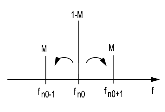
The name modelocking originates from studying this pulse formation process in the frequency domain. Note, the term

\[-M [1 - \cos (\omega_M t)] A \nonumber \]

does generate sidebands on each cavity mode present according to

\[\begin{array} {ll} \ & {-M[1 - \cos (\omega_M t)] \exp (j \omega_{n_0} t)} \\ = & {-M \left [\exp (j \omega_{n_0} t) - \dfrac{1}{2} \exp (j (\omega_{n_0} t - \omega_M t)) - \dfrac{1}{2} \exp (j (\omega_{n_0} t + \omega_M t))\right ]} \\ = & {M\left [-\exp(j \omega_{n_0} t) + \dfrac{1}{2}(j \omega_{n_0 - 1} t) + \dfrac{1}{2}(j \omega_{n_0 + 1} t) \right ]} \end{array} \nonumber \]

if the modulation frequency is the same as the cavity round-trip frequency. The sidebands generated from each running mode is injected into the neighboring modes which leads to synchronisation and locking of neighboring modes, i.e. mode-locking, see Fig.5.6