
5.4: Active Mode Locking with Additional SPM
- Page ID
- 44659

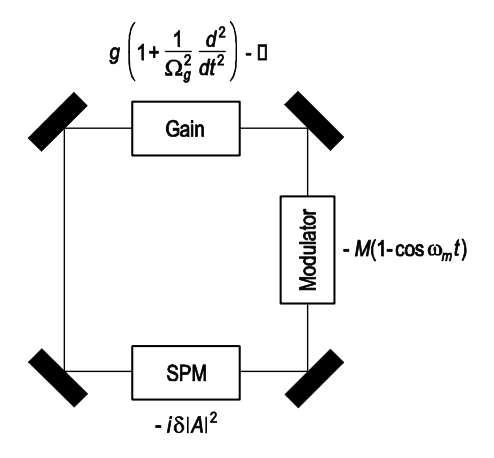
Due to the strong focussing of the pulse in the gain medium also additional self-phase modulation can become important. Lets consider the case of an actively mode-locked laser with additional SPM, see Figure 5.7. One can write down the corresponding master equation
\[T_R \dfrac{\partial A}{\partial T} = \left [g(T) + D_g \dfrac{\partial^2}{\partial t^2} - l - M_s t^2 - j \delta |A|^2 \right ] A.\label{eq5.4.1} \]
Unfortunately, there is no analytic solution to this equation. But it is not difficult to guess what will happen in this case. As long as the SPM is not excessive, the pulses will experience additional self-phase modulation, which creates a chirp on the pulse. Thus one can make an ansatz with a chirped Gaussian similar to (5.3.4) for the steady state solution of the master equation (\(\ref{eq5.4.1}\))
\[A_0 (t) = Ae^{-\tfrac{t^2}{2\tau_a^2} (1 + j \beta) j \Psi T/T_R} \nonumber \]
Note, we allow for an additional phase shift per roundtrip \(\Psi\), because the added SPM does not leave the phase invariant after one round-trip. This is still a steady state solution for the intensity envelope. Substitution into the master equation using the intermediate result
\[\dfrac{\partial ^2}{\partial t^2} A_0 (t) = \left \{\dfrac{t^2}{\tau_a^4} (1 + j\beta)^2 - \dfrac{1}{\tau_a^2} (1 + j \beta) \right \} A_0 (t). \nonumber \]
leads to
\[j \Psi A_0 (t) = \left \{g - l + D_g \left [\dfrac{t^2}{\tau_a^4} (1 + j\beta)^2 - \dfrac{1}{\tau_a^2} (1 + j \beta) \right ] - M_s t^2 - j \delta |A|^2 e^{-\tfrac{t^2}{\tau_a^2}} \right \} A_0 (t). \nonumber \]
To find an approximate solution we expand the Gaussian in the bracket, which is a consequency of the SPM to first order in the exponent.
\[j \Psi = g- l + D_g \left [\dfrac{t^2}{\tau_a^4} (1 + j\beta)^2 - \dfrac{1}{\tau_a^2} (1 + j \beta) \right ] - M_s t^2 - j \delta |A|^2 \left (1 - \dfrac{t^2}{\tau_a^2} \right ). \nonumber \]
This has to be fulfilled for all times, so we can compare coefficients in front of the constant terms and the quadratic terms, which leads to two complex conditions. This leads to four equations for the unknown pulsewidth \(\tau_a\), chirp \(\beta\), round-trip phase \(\Psi\) and the necessary excess gain \(g - l\). With the nonlinear peak phase shift due to SPM, \(\phi_0 = \delta |A|^2\). Real and Imaginary parts of the quadratic terms lead to
\[0 = \dfrac{D_g}{\tau_a^4} (1 - \beta^2) - M_s, \nonumber \]
\[0 = 2 \beta \dfrac{D_g}{\tau_a^4} + \dfrac{\phi_0}{\tau_a^2}, \nonumber \]
and the constant terms give the excess gain and the additional round-trip phase.
\[g - l = \dfrac{D_g}{\tau_a^2}, \nonumber \]
\[\Psi = D_g \left [-\dfrac{1}{\tau_a^2} \beta \right ] - \phi_0. \nonumber \]
The first two equations directly give the chirp and pulse width.
\[\beta = -\dfrac{\phi_0 \tau_a^2}{2D_g} \nonumber \]
\[\tau_a^4 = \dfrac{D_g}{M_s + \tfrac{\phi_0^2}{4D_g}}. \nonumber \]
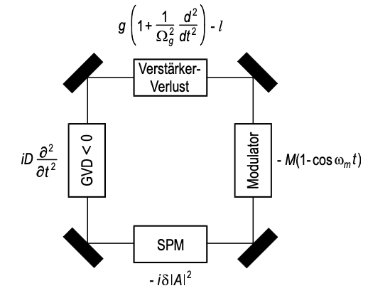
However, one has to note, that this simple analysis does not give any hint on the stability of these approximate solution. Indeed computer simulations show, that after an additional pulse shorting of about a factor of 2 by SPM beyond the pulse width already achieved by pure active mode-locking on its own, the SPM drives the pulses unstable [5]. This is one of the reasons, why very broadband laser media, like Ti:sapphire, can not simply generate femtosecond pulses via active medolocking. The SPM occuring in the gain medium for very short pulses drives the modelocking unstable. Additional stabilization measures have to be adopted. For example the addition of negative group delay dispersion might lead to stable soliton formation in the presence of the active modelocker.