5.7: Active Modelocking with Detuning

So far, we only considered the case of perfect synchronism between the round-trip of the pulse in the cavity and the external modulator. Technically, such perfect synchronism is not easy to achieve. One way would be to do regenerative mode locking, i.e. a part of the output signal of the modelocked laser is detected, the beatnote at the round-trip frequency is filtered out from the detector, and sent to an amplifier, which drives the modulator. This procedure enforces synchronism if the cavity length undergoes fluctuations due to acoustic vibrations and thermal expansion.

Nevertheless, it is interesting to know how sensitive the system is against detuning between the modulator and the resonator. It turns out that this is a physically and mathematically rich situation, which applies to many other phenomena occuring in externally driven systems, such as the transition from laminar to turbulent flow in hydrodynamics. This transition has puzzled physicists for more than a hundred years [1]. During the last 5 to 10 years, a scenario for the transition to turbulence has been put forward by Trefethen and others [2]. This model gives not only a quantitative description of the kind of instability that leads to a transition from laminar, i.e. highly ordered dynamics, to turbulent flow, i.e. chaotic motion, but also an intuitive physical picture why turbulence is occuring. Such a picture is the basis for many laser instabilities especially in synchronized laser systems. According to this theory, turbulence is due to strong transient growth of deviations from a stable stationary point of the system together with a non-linear feedback mechanism. The nonlinear feedback mechanism couples part of the amplified perturbation back into the initial perturbation. Therefore, the perturbation experiences strong growth repeatedly. Once the transient growth is large enough, a slight perturbation from the stable stationary point renders the system into turbulence. Small perturbations are always present in real systems in the form of system intrinsic noise or environmental noise and, in computer simulations, due to the finite precision. The predictions of the linearized stability analysis become meaningless in such cases. The detuned actively modelocked laser is an excellent example of such a system, which in addition can be studied analytically. The detuned case has been only studied experimentally [3][4] or numerically [5] so far. Here, we consider an analytical approach. Note, that this type of instability can not be detected by a linear stability analysis which is widely used in laser theories and which we use in this course very often to prove stable pulse formation. One has to be aware that such situations may arise, where the results of a linearized stability analysis have only very limited validity.

The equation of motion for the pulse envelope in an actively modelocked laser with detuning can be writen as

\[T_M \dfrac{\partial A(T, t)}{\partial T} = \left [g(T) - l + D_f \dfrac{\partial^2}{\partial t^2} - M(1 - \cos (\omega_M t)) + T_d \dfrac{\partial}{\partial t} \right ] A(T, t).\label{eq5.7.1} \]

Here, \(A(T,t)\) is the pulse envelope as before. There is the time \(T\) which is coarse grained on the time scale of the resonator round-trip time \(T_R\) and the time \(t\), which resolves the resulting pulse shape. The saturated gain is denoted by \(g(T)\) and left dynamical, because we no longer assume that the gain and field dynamics reaches a steady state eventually. The curvature of the intracavity losses in the frequency domain, which limit the bandwidth of the laser, is given by \(D_f\) and left fixed for simplicity. \(M\) is the depth of the loss modulation introduced by the modulator with angular frequency \(\omega_M = 2\pi /T_M\), where \(T_M\) is the modulator period. Note that Eq.(\(\ref{eq5.7.1}\)) describes the change in the pulse between one period of modulation. The detuning between resonator round-trip time and the modulator period is \(T_d = T_M − T_R\).This detuning means that the pulse hits the modulator with some temporal off-set after one round-trip, which can be described by adding the term \(T_d \dfrac{\partial}{\partial A} A\) inthe master equation.The saturated gain \(g\) obeys a separate ordinary differential equation

\[\dfrac{\partial g (T)}{\partial T} = - \dfrac{g(T) - g_0}{\tau_L} - g \dfrac{W(T)}{P_L}. \nonumber \]

As before, \(g_0\) is the small signal gain due to the pumping, \(P_L\) the saturation power of the gain medium, \(\tau_L\) the gain relaxation time and \(W (T) = \int |A(T,t)|^2\ dt\) the total field energy stored in the cavity at time \(T\).

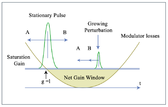
As before, we expect pulses with a pulse width much shorter than the round-trip time in the cavity and we assume that they still will be placed in time near the position where the modulator introduces low loss (Figure 5.15), so that we can still approximate the cosine by a parabola

\[T_M \dfrac{\partial A}{\partial T} = \left [g - l + D_f \dfrac{\partial ^2}{\partial t^2} - M_s t^2 + T_d \dfrac{\partial}{\partial t} \right ] A.\label{eq5.7.3} \]

Figure 5.15: Drifting pulse dynamics in a detuned actively modelocked laser for the situation, where the modulator period is larger than the cavity round-trip time. The displacement A is caused by the mismatch between the cavity round-trip time and the modulator period. The displacement B is due to unequal losses experienced by the front and the back of the pulse in the modulator. The gain saturates to a level where a possible stationary pulse experiences no net gain or loss, which opens up a net gain window following the pulse. Perturbations within that window get amplified while drifting towards the stationary pulse.. Figure by MIT OCW.

Here, \(M_s = M\omega_M^2 /2\) is the curvature of the loss modulation at the point of minimum loss as before. The time t is now allowed to range from \(-\infty\) to \(+\infty\), since the modulator losses make sure that only during the physically allowed range \(-T_R/2 \ll t \ll T_R/2\) radiation can build up.

In the case of vanishing detuning, i.e. \(T_d = 0\), the differential operator on the right side of (\(\ref{eq5.7.3}\)), which generates the dynamics and is usually called a evolution operator \(\hat{L}\), correspondes to the Schrödinger operator of the harmonic oscillator. Therefore, it is useful to introduce the creation and annihilation operators

\[\hat{a} = \dfrac{1}{\sqrt{2}} \left (\dfrac{\tau_a \partial}{\partial t} + \dfrac{t}{\tau_a} \right ), \hat{a}^{\dagger} = \dfrac{1}{\sqrt{2}} \left (\dfrac{\tau_a \partial}{\partial t} + \dfrac{t}{\tau_a} \right ), \nonumber \]

with \(\tau_a = \sqrt[4]{D_f/M_s}\). The evolution operator \(\hat{L}\) is then given by

\[\hat{L} = g- l - 2 \sqrt{D_f M_s} \left (\hat{a}^{\dagger} \hat{a} + \dfrac{1}{2} \right )\label{eq5.7.5} \]

and the evolution equation (\(\ref{eq5.7.3}\)) can be written as

\[T_M \dfrac{\partial A}{\partial T} = \hat{L} A. \nonumber \]

Consequently, the eigensolutions of this evolution operator are the Hermite-Gaussians, which we used already before

\[A_n (T, t) = u_n (t) e^{\lambda_n T/ T_M} \nonumber \]

\[u_n(t) = \sqrt{\dfrac{W_n}{2^n \sqrt{\pi} n! \tau_a}} H_n (t/\tau_a) e^{-\tfrac{t^2}{2\tau_a^2}}\label{eq5.7.8} \]

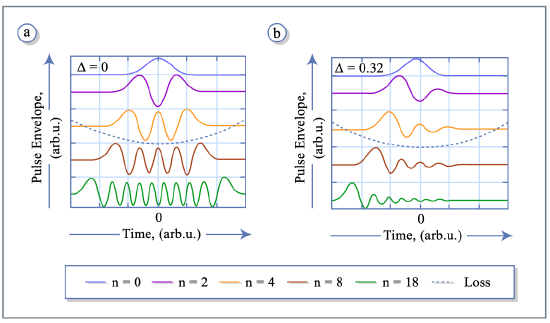
and \(\tau_a\) is the pulsewidth of the Gaussian.(see Figure 5.16a)

Figure 5.16: Lower order eigenmodes of the linearized system for zero detuning, \(\Delta = 0\), (a) and for a detuning, \(\Delta = 0.32\), in (b).. Figure by MIT OCW.

The eigenmodes are orthogonal to each other because the evolution operator is hermitian in this case.

The round-trip gain of the eigenmode \(u_n (t)\) is given by its eigenvalue (or in general by the real part of the eigenvalue) which is given by \(\lambda_n = g_n - l - 2 \sqrt{D_f M_s} (n + 0.5)\) where \(g_n = g_0 \left (1 + \tfrac{W_n}{P_L T_R} \right )^{-1}\), with \(W_n = \int |u_n (t)|^2 dt\). The eigenvalues prove that, for a given pulse energy, the mode with \(n = 0\), which we call the ground mode, experiences the largest gain. Consequently, the ground mode will saturate the gain to a value such that \(\lambda_0 = 0\) in steady state and all other modes experience net loss, \(\lambda_n < 0\) for \(n > 0\), as discussed before. This is a stable situation as can be shown rigorously by a linearized stability analysis [6]. Thus active modelocking with perfect synchronization produces Gaussian pulses with a 1/\(e\)-half width of the intensity profile given by \(\tau_a\).

In the case of non zero detuning \(T_d\), the situation becomes more complex. The evolution operator, (\(\ref{eq5.7.5}\)), changes to

\[\hat{L}_D = g - l - 2 \sqrt{D_fM_s} \left [(\hat{a}^{\dagger} - \Delta)(\hat{a} + \Delta) + (\dfrac{1}{2} + \Delta^2) \right ] \nonumber \]

with the normalized detuning

\[\Delta = \dfrac{1}{2\sqrt{2D_fM_s}} \dfrac{T_d}{\tau_a}.\label{eq5.7.10} \]

Introducing the shifted creation and annihilation operators, \(\hat{b}^{\dagger} = \hat{a}^{\dagger} + \Delta\) and \(\hat{b} = \hat{a} + \Delta\), respectively, we obtain

\[\hat{L}_D = \Delta_g - 2 \sqrt{D_fM_s} (\hat{b}^{\dagger} \hat{b} - 2 \Delta \hat{b}) \nonumber \]

with the excess gain

\[\Delta g = g - l - 2 \sqrt{D_f M_s} (\dfrac{1}{2} + \Delta^2) \nonumber \]

due to the detuning. Note, that the resulting evolution operator is not any longer hermitian and even not normal, i.e. \([A, A^{\dagger}] \ne 0\), which causes the eigenmodes to become nonnormal [8]. Nevertheless, it is an easy excercise to compute the eigenvectors and eigenvalues of the new evolution operator in terms of the eigenstates of \(\hat{b}^{\dagger} \hat{b}, | l \rangle\), which are the Hermite Gaussians centered around \(\Delta\). The eigenvectors \(| \varphi_n \rangle\) to \(\hat{L}_D\) are found by the ansatz

\[|\varphi_n \rangle = \sum_{l = 0}^{n} c_l^n |l \rangle, \text{ with } c_{l +1}^{n} = \dfrac{n - l}{2 \Delta \sqrt{l + 1}} c_l^n.\label{eq5.7.13} \]

The new eigenvalues are \(\lambda_n = g_n - l - 2\sqrt{D_fM_s} (\Delta^2 + n + 0.5)\). By inspection, it is again easy to see, that the new eigenstates form a complete basis in \(L_2 (\mathbb{R})\). However, the eigenvectors are no longer orthogonal to each other. The eigensolutions as a function of time are given as a product of a Hermite Polynomial and a shifted Gaussian \(u_n (t) = \langle t | \varphi_n \rangle \sim H_n (t/\tau_a) \exp [-\tfrac{(t - \sqrt{2} \Delta_{\tau_a})^2}{2 \tau_a^2}]\). Again, a linearized stability analysis shows that the ground mode, i.e. \(|\varphi_0 \rangle\), a Gaussian, is a stable stationary solution. Surprisingly, the linearized analysis predicts stability of the ground mode for all values of the detuning in the parabolic modulation and gain approximation. This result is even inde- pendent from the dynamics of the gain, i.e. the upper state lifetime of the active medium, as long as there is enough gain to support the pulse. Only the position of the maximum of the ground mode, \(\sqrt{2} \Delta \cdot \tau_a\), depends on the normalized detuning.

Figure 5.15 summarizes the results obtained so far. In the case of detuning, the center of the stationary Gaussian pulse is shifted away from the position of minimum loss of the modulator. Since the net gain and loss within one round-trip in the laser cavity has to be zero for a stationary pulse, there is a long net gain window following the pulse in the case of detuning due to the necessary excess gain. Figure 2 shows a few of the resulting lowest order eigenfunctions for the case of a normalized detuning \(\Delta = 0\) in (a) and \(\Delta = 0.32\) in (b). These eigenfunctions are not orthogonal as a result of the nonnormal evolution operator

Dynamics of the Detuned Actively Mode-locked Laser

To get insight into the dynamics of the system, we look at computer simulations for a \(\ce{Nd:YLF}\) Laser with the parameters shown in Table 5.3 Figures

Table 5.3: Data used in the simulations of a \(\ce{Nd:YLF}\) laser.

\(E_L = 366 \ \mu J\)	\(g_0 = 0.79\)
\(\tau_L = 450 \ \mu s\)	\(M_s = 2.467 \cdot 10^{17} s^{-2}\)
\(\Omega_g = 1.12 THz\)	\(D_g = 2 \cdot 10^{-26} s^2\)
\(T_R = 4\ ns\)	\(\tau_a = 17 \ ps\)
\(l = 0.025\)	\(\lambda_0 = 1.047\ \mu m\)
\(M = 0.2\)

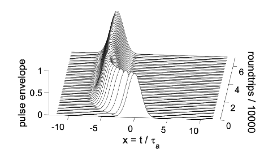
5.17 show the temporal evolution of the coefficient cn,when the master equation is decomposed into Hermite Gaussians centered at \(t=0\) according to Equation (\(\ref{eq5.7.8}\)).

\[A(T, t) = \sum_{n = 0}^{\infty} c_n (T) u_n (t)\nonumber \]

Figure 5.17: Coefficients of the envelope in a Hermite-Gaussian-Basis, as a function of resonator round-trips. The normalized detuning is \(\Delta = 3.5\). The simulation starts from the steady state without detuning. The curve starting at 1 is the ground mode. To describe a shifted pulse, many modes are necessary.

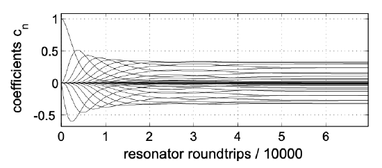
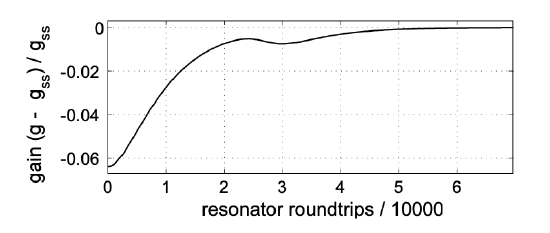
Figure 5.18 and 5.19 shows the deviation from the steady state gain and the pulse envelope in the time domain for a normalized detuning of \(\Delta = 3.5\).

Figure 5.18: Gain as a function of the number of roundtrips. It changes to a higher level.

Figure 5.19: Temporal evolution of the pusle envelope. The pulse shifts slowly into the new equilibrium position at \(\sqrt{2} \Delta = 4.9\) in agreement with the simulation.

Figures 5.20 to 5.22 show the same quantities for a slightly higher normalized detuning of \(\Delta = 4\).

Figure 5.20: Temporal evolution of the coefficients in a Hermite-Gaussian Basis at a normalized detuning of \(\Delta = 4\). Almost peridoically short interrupting events of the otherwise regular motion can be easily recognized (Intermittent Behavior). Over an extended period time between such events the laser approaches almost a steady state.

Figure 5.22: Time evolution of pulse envelope.

Figure 5.21: Temporal evolution of deviation from quasi steady state gain.

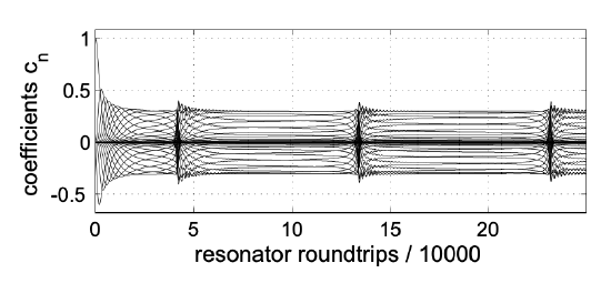
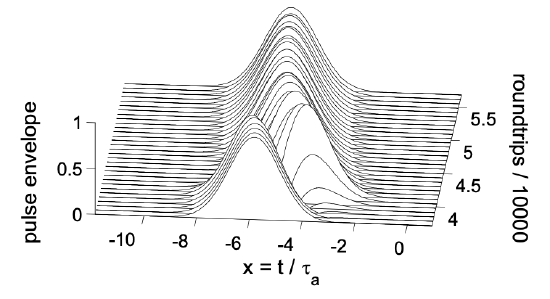
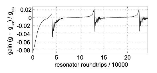
The pictures clearly show that the system does not approach a steady state anymore, but rather stays turbulent, i.e. the dynamics is chaotic.

Nonnormal Systems and Transient Gain

To get insight into the dynamics of a nonnormal time evolution, we consider the following two-dimensional nonnormal system

\[\dfrac{du}{dt} = Au,\ u(0) = u_0,\ u(t) = e^{At} u_0 \nonumber \]

Figure 5.23: Decomposition of an initial perturbation in the eigen basis.

with

\[A = \left (\begin{matrix} -\tfrac{1}{2} & \tfrac{a}{2} \\ 0 & -1 \end{matrix} \right ) \Rightarrow A^{\dagger} = \left (\begin{matrix} -\tfrac{1}{2} & 0 \\ \tfrac{a}{2} & -1 \end{matrix} \right ), [A, A^{\dagger}] = \dfrac{a}{4} \left (\begin{matrix} a & 1 \\ 1 & a \end{matrix} \right ) \ne 0. \nonumber \]

The parameter \(a\) scales the strength of the nonnormality, similar to the detuning \(\Delta\) in the case of a modelocked laser or the Reynolds number in hydrodynamics, where the linearized Navier-Stokes Equations constitute a nonnormal system.

The eigenvalues and vectors of the linear system are

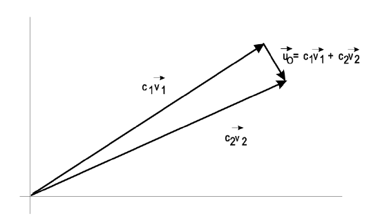
\[\lambda_1 = - \dfrac{1}{2}, v_1 = \left (\begin{matrix} 1 \\ 0 \end{matrix} \right ), \lambda_2 = -1, v_2 = \dfrac{1}{\sqrt{1 + a^2}} \left (\begin{matrix} a \\ -1 \end{matrix} \right ) \nonumber \]

The eigenvectors build a complete system and every initial vector can be decomposed in this basis. However, for large a, the two eigenvectors become more and more parallel, so that a decomposition of a small initial vector almost orthogonal to the basis vectors needs large components (Figure 5.23)

The solution is

\[u(t) = e^{At} u_0 = c_1 e^{-t/2} \vec{v}_1 + c_2 e^{-t} \vec{v}_2.\nonumber \]

Since the eigenvalues are negative, both contributions decay, and the system is stable. However, one eigen component decays twice as fast than the other one. Of importance to us is the transient gain that the system is showing due to the fact of near parallel eigen vectors. Both coefficients \(c_1\) and \(c_2\) are large. When one of the components decays, the other one is still there and the resulting vector

\[u(t \to 2) \approx c_1 e^{-1} \vec{v}_1.\nonumber \]

can be much larger then the initial perturbation during this transient phase.

This is transient gain. It can become arbitrarily large for large \(a\).

Nonormal Behavior of the Detuned Laser

The nonnormality of the operator, \([\hat{L}_D, \hat{L}_D^{\dagger} \sim \Delta\), increases with detuning. Figure 5.24 shows the normalized scalar products between the eigenmodes for different values of the detuning

\[C(m, n) = \left |\dfrac{\langle \varphi_m |\varphi_n \rangle}{\sqrt{\langle \varphi_m |\varphi_m \rangle \langle \varphi_n |\varphi_n \rangle}} \right |. \nonumber \]

The eigenmodes are orthogonal for zero detuning. The orthogonality vanishes with increased detuning. The recursion relation (\(\ref{eq5.7.13}\)) tells us that the overlap of the new eigenmodes with the ground mode increases for increasing detuning. This corresponds to the parallelization of the eigenmodes of the linearzed problem whihc leads to large transient gain, \(|| e^{\hat{L}_D t}||\), in a nonnormal situation [2]. Figure 5.24d shows the transient gain for an initial perturbation from the stationary ground mode calculated by numerical simulations of the linearized system using an expansion of the linearized system in terms of Fock states to the operator \(\hat{b}\). A normalized detuning of \(\Delta = 3\) already leads to transient gains for perturbations of the order of 106 within 20, 000 round-trips which lead to an enormous sensitivity of the system against perturbations. An analytical solution of the linearized system neglecting the gain saturation shows that the transient gain scales with the detuning according to \(\exp(2\Delta^2)\). This strong super exponential growth with increasing detuning determines the dynamics completely.

Image removed due to copyright restrictions.

Please see:
Kaertner, F. X., et al. "Turbulence in Mode-locked Lasers". Physical Review Letters 82, no. 22 (May 1999): 4428-4431.

Figure 5.24: Scalar products of eigenvectors as a function of the eigenvector index for the cases \(\Delta = 0\) shown in (a), \(\Delta = 1\) in (b) and \(\Delta = 3\) in (c). (d) shows the transient gain as a funtion of time for these detunings computed and for \(\Delta = 2\), from the linearized system dynamics.

Image removed due to copyright restrictions.

Please see:
Kaertner, F. X., et al. "Turbulence in Mode-locked Lasers". Physical Review Letters 82, no. 22 (May 1999): 4428-4431.

Figure 5.25: Critical detuning obtained from numerical simulations as a function of the normalized pumping rate and cavity decay time divided by the upper-state lifetime. The crititcal detuning is almost independent of all laser parameters shown. The mean critical detuning is \(\Delta \approx 3.65\).

Figure 5.25 shows the surface of the transition to turbulence in the pa- rameter space of a \(\ce{Nd:YLF}\) laser, i.e. critical detuning \(\Delta\), the pumping rate \(r = g_0/l\) and the ratio between the cavity decay time \(T_{cav} = T_R/l\) and the upper state lifetime \(\tau_L\). In this model, we did not inlcude the spontaneous emission.

The transition to turbulence always occurs at a normalized detuning of about \(\Delta \approx 3.7\) which gives a transient gain \(\exp(2\Delta^2) = 10^{12}\). This means that already uncertainties of the numerical integration algorithm are amplified to a perturbation as large as the stationary state itself.To prove that the system dynamics becomes really chaotic, one has to compute the Liapunov coefficient [9]. The Liapunov coefficient describes how fast the phase space trajectores separate from each other, if they start in close proximity. It is formally defined in the following way. Two trajectories \(y(t)\) and \(z(t)\) start in close vicinity at \(t = t_0\)

\[||y(t_0) - z(t_0)|| = \epsilon = 10^{-4}. \nonumber \]

Then, the system is run for a certain time \(\Delta t\) and the logarithmic growth rate, i.e. Liapunov coefficient, of the distance between both trajectories is evaluated using

\[\lambda_0 = \ln \left (\dfrac{||y(t_0 + \Delta t) - z (t_0 + \Delta t) ||}{\epsilon} \right )\label{eq5.7.19} \]

For the next iteration the trajectory \(z(t)\) is rescaled along the distance between \(y(t_0 + \Delta t)\) and \(z(t_0 + \Delta t)\) according to

\[z(t_1) = y(t_0 + \Delta t) + \epsilon \dfrac{y(t_0 + \Delta t) - z (t_0 + \Delta t)}{||y(t_0 + \Delta t) - z (t_0 + \Delta t) ||}. \nonumber \]

The new points of the trajectories \(z (t_1 + \Delta t)\) and \(y (t_1 + \Delta t) = y(t_0 + 2\Delta t)\) are calculated and a new estimate for the Liapunov coefficient \(\lambda_1\) is calculated using Eq.(\(\ref{eq5.7.19}\)) with new indices. This procedure is continued and the Liapunov coefficient is defined as the average of all the approximations over a long enough iteration, so that its changes are below a certain error bound from iteration to iteration.

\[\lambda = \dfrac{1}{N} \sum_{n = 0}^{N} \lambda_n \nonumber \]

Figure 5.26 shows the Liapunov coefficient of the \(\ce{Nd:YLF}\) laser discussed above, as a function of the normlized detuning. When the Liapunov coefficient becomes positive, i.e. the system becomes exponentially sensitive to small changes in the initial conditions, the system is called chaotic. The graph clearly indicates that the dynamics is chaotic above a critical detuning of about \(\Delta_c \approx 3.7\).

Image removed due to copyright restrictions.

Please see:
Kaertner, F. X., et al. "Turbulence in Mode-locked Lasers". Physical Review Letters 82, no. 22 (May 1999): 4428-4431.

Figure 5.26: Liapunov coefficient over normalized detuning.

In the turbulent regime, the system does not reach a steady state, because it is nonperiodically interrupted by a new pulse created out of the net gain window, see Figure 5.15, following the pulse for positive detuning. This pulse saturates the gain and the nearly formed steady state pulse is destroyed and finally replaced by a new one. The gain saturation provides the nonlinear feedback mechanism, which strongly perturbs the system again, once a strong perturbation grows up due to the transient linear amplification mechanism.

The critical detuning becomes smaller if additional noise sources, such as the spontaneous emission noise of the laser amplifier and technical noise sources are taken into account. However, due to the super exponential growth, the critical detuning will not depend strongly on the strength of the noise sources. If the spontaneous emission noise is included in the simulation, we obtain the same shape for the critical detuning as in Figure 5.25, however the critical detuning is lowered to about \(\Delta_c \approx 2\). Note that this critical detuning is very insensitive to any other changes in the parameters of the system. Therefore, one can expect that actively mode-locked lasers without regenerative feedback run unstable at a real detuning, see (\(\ref{eq5.7.10}\)) given by

\[T_d = 4\sqrt{2D_f M_s} \tau_a \nonumber \]

For the above \(\ce{Nd:YLF}\) laser, using the values in Table 5.3 results in a relative precision of the modulation frequency of

\[\dfrac{T_d}{T_R} = 1.7 \cdot 10^{-6} \nonumber \]

The derived value for the frequency stability can easily be achieved and maintained with modern microwave synthesizers. However, this requires that the cavity length of \(\ce{Nd:YLF}\) laser is also stable to this limit. Note that the thermal expansion coefficient for steel is \(1.6 \cdot 10^{-5}/K\).

Bibliography

[1] Lord Kelvin, Philos. Mag. 24, 188 (1887); A. Sommerfeld, Int. Mathem. Kongr. Rom 1908, Vol. III, S. 116; W. M. F. Orr, Proc. Irish Acad. 27, (1907).

[2] L. Trefethen, A. Trefethen, S. C. Reddy u. T. Driscol, Science 261, 578 (1993); S. C. Reddy, D. Henningson, J. Fluid Mech. 252, 209 (1993); Phys. Fluids 6, 1396 (1994); S. Reddy et al., SIAM J. Appl. Math. 53; 15 (1993); T. Gebhardt and S. Grossmann, Phys. Rev. E 50, 3705 (1994).

[3] H. J. Eichler, Opt. Comm. 56, 351 (1986). H. J. Eichler, I. G. Koltchanov and B. Liu, Appl. Phys. B 61, 81 (1995).

[4] U. Morgner and F. Mitschke, Phys. Rev.A54, 3149 (1997).

[5] H. J. Eichler, I. G. Koltchanov and B. Liu, Appl. Phys. B 61, 81 - 88 (1995).

[6] H. A. Haus, IEEE JQE 11, 323 (1975).

[7] H. A. Haus, D. J. Jones, E. P. Ippen and W. S. Wong, Journal of Light- wave Technology, 14, 622 (1996).

[8] G. Bachman and L. Narici, ”Functional Analysis”, New York, Academic Press (1966).

[9] A. Wolf, J. B. Swift, H. L. Swinney and J. A. Vastano, Physica D 16, 285 (1985).