1.4: Flux and Divergence

If we measure the total mass of fluid entering the volume in Figure 1-13 and find it to be less than the mass leaving, we know that there must be an additional source of fluid within the pipe. If the mass leaving is less than that entering, then

Figure 1-13 The net flux through a closed surface tells us whether there is a source or sink within an enclosed volume.

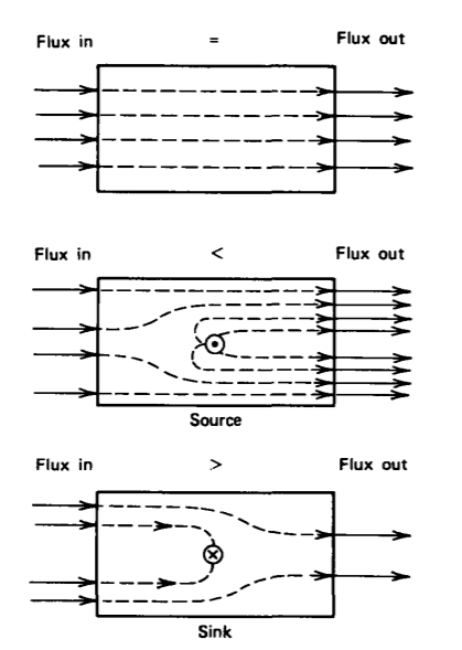
there is a sink (or drain) within the volume. In the absence of sources or sinks, the mass-of fluid leaving equals that entering so the flow lines are continuous. Flow lines originate at a source and terminate at a sink.

Flux

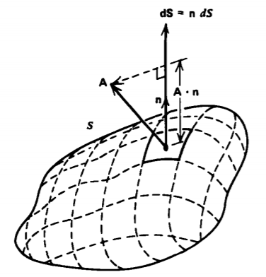
We are illustrating with a fluid analogy what is called the flux (\(\Phi\) of a vector A through a closed surface:

\[\Phi = \oint_{S}A \cdot \bf{dS} \]

The differential surface element dS is a vector that has magnitude equal to an incremental area on the surface but points in the direction of the outgoing unit normal n to the surface S, as in Figure 1-14. Only the component of A perpendicular to the surface contributes to the flux, as the tangential component only results in flow of the vector A along the surface and not through it. A positive contribution to the flux occurs if A has a component in the direction of dS out from the surface. If the normal component of A points into the volume, we have a negative contribution to the flux.

If there is no source for A within the volume V enclosed by the surface S, all the flux entering the volume equals that leaving and the net flux is zero. A source of A within the volume generates more flux leaving than entering so that the flux is positive (\(\Phi\)>0) while a sink has more flux entering than leaving so that (\(\Phi\)< 0.)

Figure 1-14 The flux of a vector A through the closed surface S is given by the surface integral of the component of A perpendicular to the surface S. The differential vector surface area element dS is in the direction of the unit normal n.

Thus we see that the sign and magnitude of the net flux relates the quantity of a field through a surface to the sources or sinks of the vector field within the enclosed volume.

Divergence

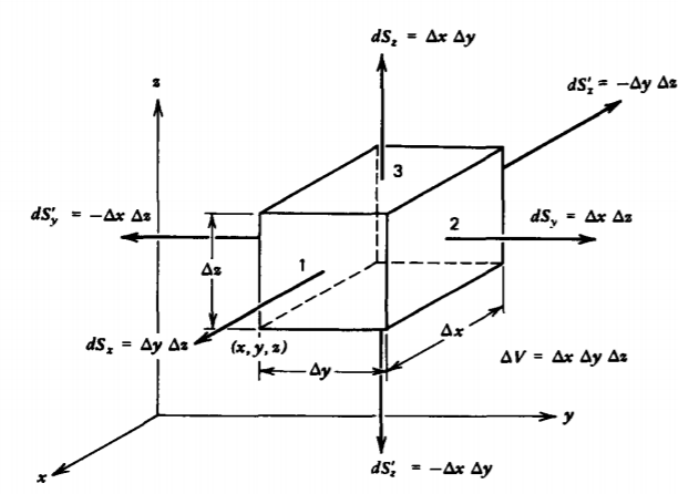
We can be more explicit about the relationship between the rate of change of a vector field and its sources by applying (1) to a volume of differential size, which for simplicity we take to be rectangular in Figure 1-15. There are three pairs of plane parallel surfaces perpendicular to the coordinate axes so that (1) gives the flux as

\[\Phi = \int_{1} A_{x}(x) dy dz = \int_{1'} A_{x}(x- \Delta x) dy dz + \int_{2}A_{y} (y + \Delta y) dx dz - \int_{2'} A_{y}(y) dx dz + \int_{3}A_{z}(z + \Delta z) dx dy - \int_{3'} A_{z}(z) dx dy \]

where the primed surfaces are differential distances behind the corresponding unprimed surfaces. The minus signs arise because the outgoing normals on the primed surfaces point in the negative coordinate directions.

Because the surfaces are of differential size, the components of A are approximately constant along each surface so that the surface integrals in (2) become pure

Figure 1-15 Infinitesimal rectangular volume used to define the divergence of a vector.

multiplications of the component of A perpendicular to the surface and the surface area. The flux then reduces to the form

\[\Phi \approx (\frac{[A_{x}(x) - A_{x}(x- \Delta x)]}{\Delta x} + \frac{[A_{y} (y + \Delta y) - A_{y} (y)]}{\Delta y} + \frac{[A_{z}(z + \Delta z) - A_{z} (z)]}{\Delta z}) \Delta x \Delta y \Delta x \]

We have written (3) in this form so that in the limit as the volume becomes infinitesimally small, each of the bracketed terms defines a partial derivative

\[\lim_{\Delta x \rightarrow 0 \\ \Delta y \rightarrow 0 \\ \Delta z \rightarrow 0} \Phi = (\frac{\partial A_{x}}{\partial x} + \frac{\partial A_{y}}{\partial y} + \frac{\partial A_{z}}{\partial z}) \Delta V \]

where \(\Delta V = \Delta x \Delta y \Delta x\) is the volume enclosed by the surface S.

The coefficient of \(\Delta V\) in (4) is a scalar and is called the divergence of A. It can be recognized as the dot product between the vector del operator of Section 1-3-1 and the vector A:

\[\textrm{div} \: \textbf{A} = \nabla \cdot \textbf{A} = \frac{\partial A_{x}}{\partial x} + \frac{\partial A_{y}}{\partial y} + \frac{\partial A_{z}}{\partial z} \]

Curvilinear Coordinates

In cylindrical and spherical coordinates, the divergence operation is not simply the dot product between a vector and the del operator because the directions of the unit vectors are a function of the coordinates. Thus, derivatives of the unit vectors have nonzero contributions. It is easiest to use the generalized definition of the divergence independent of the coordinate system, obtained from (1)-(5) as

\[\nabla \cdot A = \lim_{\Delta V \rightarrow 0} \frac{\oint_{S} \textbf{A} \cdot \textbf{dS}}{\Delta V} \]

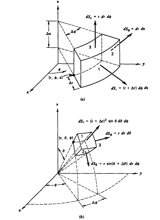
(a) Cylindrical Coordinates

In cylindrical coordinates we use the small volume shown in Figure 1-16a to evaluate the net flux as

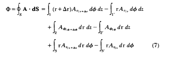
\[\Phi = \oint_{S} \textbf{A} \cdot \textbf{dS} = \int_{1} (\textrm{r} + \Delta \textrm{r}) A_{\textrm{r}_{\mid_{\textrm{r} + \Delta \textrm{r}}}} d \phi dz - \int_{1'} \textrm{r} A_{\textrm{r}_{\mid_{\textrm{r}}}} d \phi dz + \int_{2} A _{\phi_{\mid \phi + \Delta \phi}} d \textrm{r}\: dz - \int_{2'} A_{\phi_{\mid \phi}} d \textrm{r} dz + \int_{3} \textrm{r} A_{z_{\mid z + \Delta z}} d \textrm{r} d \phi - \int_{3'} \textrm{r} A_{z_{\mid_{z}}} d \textrm{r} d \phi \]

Figure 1-16 Infinitesimal volumes used to define the divergence of a vector in (a) cylindrical and (b) spherical geometries.

Again, because the volume is small, we can treat it as approximately rectangular with the components of A approximately constant along each face. Then factoring out the volume \(\Delta V = \textrm{r} \Delta \textrm{r} \Delta \phi \Delta z\) in (7),

\[\Phi \approx (\frac{[(r + \Delta r) A_{r_{\mid \textrm{r} + \Delta \textrm{r}}} -\textrm{r} A_{\textrm{r}_{\mid \textrm{r}}}]}{\textrm{r} \Delta \textrm{r}} + \frac{[A_{\phi_{\mid \phi + \Delta \phi}} - A_{\phi_{\mid_{\phi}}}]}{\textrm{r} \Delta \phi} + \frac{[A_{z_{\mid z + \Delta z}} - A_{z_{\mid z}}]}{\Delta z}) \textrm{r} \Delta \textrm{r} \: \Delta \phi \: \Delta z \]

lets each of the bracketed terms become a partial derivative as the differential lengths approach zero and (8) becomes an exact relation. The divergence is then

\[\nabla \cdot \textbf{A} = \lim_{\Delta \textrm{r} \rightarrow 0 \\ \Delta \phi \rightarrow 0 \\ \Delta x \rightarrow 0} \: \frac{\oint_{S} \textbf{A} \cdot \textbf{dS}}{\Delta V} =\frac{1}{\textrm{r}} \frac{\partial}{\partial \textrm{r}} (\textrm{r} A_{\textrm{r}}) + \frac{1}{\textrm{r}} \frac{\partial A_{\phi}}{\partial \phi} + \frac{\partial A_{z}}{\partial z} \]

(b) Spherical Coordinates

Similar operations on the spherical volume element \(\Delta V = r^{2} \sin \: \theta \: \Delta r \: \Delta \theta \: \Delta \phi\) in Figure 1-16b defines the net flux through the surfaces:

\[\Phi = \oint_{2} \textbf{A} \cdot \textbf{dS} \approx (\frac{[(r + \Delta r)^{2} A_{r_{\mid r + \Delta r}} -r^{2}A_{r_{\mid r}}]}{r^{2} \Delta r} + \frac{[A_{\theta_{\mid \theta + \Delta \theta}} \sin \: (\theta + \Delta \theta) - A_{\theta_{\mid \theta}} \: \sin \theta]}{r \: \sin \: \theta \: \Delta \theta} + \frac{[A_{\phi_{\mid \phi + \Delta \phi}} - A_{\phi_{\mid \phi}}]}{r \: \sin \: \theta \: \Delta \phi}) r^{2} \: \sin \theta \: \Delta r \: \Delta \theta \: \Delta \phi \]

The divergence in spherical coordinates is then

\[\nabla \cdot \textbf{A} = \lim_{\Delta r \rightarrow 0 \\ \Delta \theta \rightarrow 0 \\ \Delta \phi \rightarrow 0} \frac{\oint_{S} \textbf{A} \cdot \textbf{dS}}{\Delta V} = \frac{1}{r^{2}} \frac{\partial}{\partial r} (r^{2} A_{r}) + \frac{1}{r \: \sin \theta} \frac{\partial}{\partial \theta}(A_{\theta} \sin \: \theta) + \frac{1}{r \: \sin \: \theta} \frac{\partial A_{\partial}}{\partial \phi} \]

Divergence Theorem

If we now take many adjoining incremental volumes of any shape, we form a macroscopic volume V with enclosing surface S as shown in Figure 1-17a. However, each interior common surface between incremental volumes has the flux leaving one volume (positive flux contribution) just entering the adjacent volume (negative flux contribution) as in Figure 1-17b. The net contribution to the flux for the surface integral of (1) is zero for all interior surfaces. Nonzero contributions to the flux are obtained only for those surfaces which bound the outer surface S of V. Although the surface contributions to the flux using (1) cancel for all interior volumes, the flux obtained from (4) in terms of the divergence operation for

Figure 1-17 Nonzero contributions to the flux of a vector are only obtained across those surfaces that bound the outside of a volume. (a) Within the volume the flux leaving one incremental volume just enters the adjacent volume where (b) the outgoing normals to the common surface separating the volumes are in opposite directions.

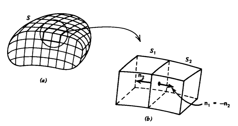
each incremental volume add. By adding all contributions from each differential volume, we obtain the divergence theorem:

\[\Phi = \oint_{S} \textbf{A} \cdot \textbf{dS} = \lim_{N \rightarrow \infty \\ \Delta V_{n} \rightarrow 0} \sum_{n=1}^{\infty} (\nabla \cdot \textbf{A}) \Delta V_{n} = \int_{V} \nabla \cdot \textbf{A} dV \]

where the volume V may be of macroscopic size and is enclosed by the outer surface S. This powerful theorem converts a surface integral into an equivalent volume integral and will be used many times in our development of electromagnetic field theory.

Example 1-6: The Divergence Theorem

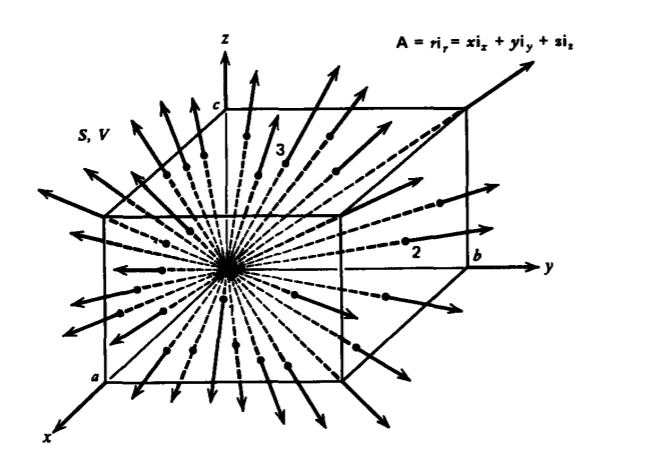
Verify the divergence theorem for the vector

\(\textbf{A} = x \textbf{i}_{x} + y \textbf{i}_{y} + z \textbf{i}_{z} = r \textbf{i}_{r}\)

by evaluating both sides of (12) for the rectangular volume shown in Figure 1-18.

Solution

The volume integral is easier to evaluate as the divergence of A is a constant

\(\nabla \cdot \textbf{a} = \frac{\partial A_{x}}{\partial x} + \frac{\partial A_{y}}{\partial y} + \frac{\partial A_{z}}{\partial z} = 3\)

Figure 1-18 The divergence theorem is verified in Example 1-6 for the radial vector through a rectangular volume.

(In spherical coordinates \(\nabla \cdot \textbf{A} = (1/r^{2})(\partial/\partial r)(r^{3}) = 3\) so that the volume integral in (12) is

\(\int_{V} \nabla \cdot \textbf{A} dV = 3abc\)

The flux passes through the six plane surfaces shown:

\(\Phi = \oint_{S} \textbf{A} \cdot \textbf{dS} = \int_{1} \underbrace{A_{x}(a)}_{a} dy dz - \int_{1'} \underbrace{A_{x}(0))}_{0} \nearrow ^{0} dy dz \\ + \int_{2} \underbrace{A_{y}(b)}_{b} dx dz - \int_{2'} \underbrace{A_{y}(0)}_{0} \nearrow ^{0} dx dz \\ + \int_{3} \underbrace{A_{z}(c)}_{c} dx dy - \int_{3'} \underbrace{A_{z}(0)}_{0} \nearrow^{0} dx dy = 3abc\)

which verifies the divergence theorem.