1.3: The Gradient and the Del Operator

Gradient

Often we are concerned with the properties of a scalar field f(x, y, z) around a particular point. The chain rule of differentiation then gives us the incremental change df in f for a small change in position from (x, y, z) to (x + dx, y + dy, z + dz):

\[df = \frac{\partial f}{\partial x} dx + \frac{\partial f}{\partial y} dy + \frac{\partial f}{\partial z} dz \]

If the general differential distance vector dl is defined as

\[\textbf{dl} = dx \textbf{i}_{z} + dy \textbf{i}_{y} + dz \textbf{i}_{z} \]

(1) can be written as the dot product:

\[df = (\frac{\partial f}{\partial x} \textbf{i}_{x} + \frac{\partial f}{\partial y} \textbf{i}_{y} + \frac{\partial f}{\partial z} \textbf{i}_{z}) \cdot \textbf{dl} \\ = \textrm{grad} \: f \cdot \textbf{dl} \]

where the spatial derivative terms in brackets are defined as the gradient of f:

\[\textrm{grad } f = \nabla f = \frac{\partial f}{\partial x} \textbf{i}_{x} + \frac{\partial f}{\partial y} \textbf{i}_{y} + \frac{\partial f}{\partial z} \textbf{i}_{z} \]

The symbol \(\nabla\) with the gradient term is introduced as a general vector operator, termed the del operator:

\[\nabla = \textbf{i}_{x} \frac{\partial}{\partial x} + \textbf{i}_{y} \frac{\partial}{\partial y} + \textbf{i}_{z} \frac{\partial}{\partial z} \]

By itself the del operator is meaningless, but when it premultiplies a scalar function, the gradient operation is defined. We will soon see that the dot and cross products between the del operator and a vector also define useful operations.

With these definitions, the change in f of (3) can be written as

\[df = \nabla f \cdot \textbf{dl} = \vert \nabla f \vert \: dl \: \cos \: \theta \]

where \(\theta\) is the angle between \(\nabla f\)Vf and the position vector dl. The direction that maximizes the change in the function f is when dl is colinear with \(\nabla f(\theta = 0)\). The gradient thus has the direction of maximum change in f. Motions in the direction along lines of constant f have \(\theta = \pi/2\) and thus by definition df=0.

Curvilinear Coordinates

Cylindrical

The gradient of a scalar function is defined for any coordinate system as that vector function that when dotted with dl gives df. In cylindrical coordinates the differential change in f(r, \(\phi\), z) is

\[df = \frac{\partial f}{\partial \textrm{r}} d \textrm{r} + \frac{\partial f}{\partial \phi} d \phi + \frac{\partial f}{\partial z} dz \]

The differential distance vector is

\[\textbf{dl} = d \textrm{r} \textbf{i}_{\textrm{r}} + \textrm{r} d \phi \: \textbf{i}_{\phi} + dz \: \textbf{i}_{z} \]

so that the gradient in cylindrical coordinates is

\[df = \nabla f \cdot \textbf{dl} \Rightarrow \nabla f = \frac{\partial f}{\partial r} \textbf{i}_{\textrm{r}} + \frac{1}{\textrm{r}} \frac{\partial f}{\partial \phi} \textrm{i}_{\phi} + \frac{\partial f}{\partial z} \textbf{i}_{\textrm{z}} \]

Spherical

Similarly in spherical coordinates the distance vector is

\[\textbf{dl} = dr \textbf{i}_{r} + r \: d \theta \: \textbf{i}_{\theta} + r \: \sin \: \theta \: d \phi \: \textbf{i}_{\phi} \]

with the differential change of f(r, \(\theta\), \(\phi\)) as

\[df = \frac{\partial f}{\partial r} dr + \frac{\partial f}{\partial \theta} d \theta + \frac{\partial f}{\partial \phi} d \phi = \nabla f \cdot \textbf{dl} \]

Using (10) in (11) gives the gradient in spherical coordinates as

\[\nabla f = \frac{\partial f}{\partial r} \textbf{i}_{r} + \frac{1}{r} \frac{\partial f}{\partial \theta} \textbf{i}_{\theta} + \frac{1}{r \: \sin \theta} \frac{\partial f}{\partial \phi} \textbf{i}_{\phi} \]

Example 1-4: Gradient

Find the gradient of each of the following functions where a and b are constants:

1. \(f = ax^{2}y + by^{3}z\)
2. \(f = a \textrm{r}^{2} \: \sin \: \phi + b \textrm{r} z \: \cos \: 2 \phi\)
3. \(f = \frac{a}{r} = br \: \sin \: \theta \: \cos \: \phi\)

Solution

(a) \(\nabla f = \frac{\partial f}{\partial x} \textbf{i}_{x} + \frac{\partial f}{\partial y} \textbf{i}_{y} + \frac{\partial f}{\partial z} \textbf{i}_{z} = 2axy \textbf{i}_{x} + (ax^{2} + 3 by^{2} z) \textbf{i}_{y} + by^{3} \textbf{i}_{z}\)

(b) \(\nabla f = \frac{\partial f}{\partial \textbf{r}} \textbf{i}_{\textrm{r}} + \frac{1}{\textrm{r}} \frac{\partial f}{\partial \phi} \textbf{i}_{\phi} + \frac{\partial f}{\partial z} \textbf{i}_{z} = (2a \textrm{r} \: \sin \: \phi + bz \: \cos \: 2 \phi) \textbf{i}_{\textrm{r}} + (a \textrm{r} \: \cos \: \phi - 2bz \: \sin \: 2 \phi) \textbf{i}_{\phi} + b \textrm{r} \: \cos \: 2 \phi \textbf{i}_{z}\)

(c) \(\nabla f = \frac{\partial f}{\partial r} \textbf{i}_{r} + \frac{1}{r} \frac{\partial f}{\partial \theta} \textbf{i}_{\theta} + \frac{1}{r \: \sin \: \theta} \frac{\partial f}{\partial \phi} \textbf{i}_{\phi} = (- \frac{a}{r^{2}} + b \: \sin \: \theta \: \cos \phi) \textbf{i}_{r} + b \: \cos \: \theta \: \cos \: \phi \textbf{i}_{\theta} - b \: \sin \: \phi \textbf{i}_{\phi}\)

Line Integral

In Section 1-2-4 we motivated the use of the dot product through the definition of incremental work as depending only on the component of force \(F\) in the direction of an object's differential displacement \(dl\). If the object moves along a path, the total work is obtained by adding up the incremental works along each small displacement on the path as in Figure 1-11. If we break the path into \(N\) small displacements

Figure 1-11 The total work in moving a body over a path is approximately equal to the sum of incremental works in moving the body each small incremental distance dl. As the differential distances approach zero length, the summation becomes a line integral and the result is exact.

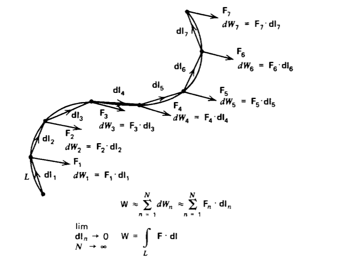
dl₁, dl₂, ..., dl_N, the work performed is approximately

\[W \approx \textbf{F}_{1} \cdot \textbf{dl}_{1} + \textbf{F}_{2} \cdot \textbf{dl}_{2} + \textbf{F}_{3} \cdot \textbf{dl}_{3} + ... + \textbf{F}_{N} \cdot \textbf{dl}_{N} \approx \sim_{n=1}^{N} \: \textbf{F}_{n} \cdot \textbf{dl}_{n} \]

The result becomes exact in the limit as \(N\) becomes large with each displacement \(dl\) becoming infinitesimally small:

\[W = \lim_{N\rightarrow \infty \\ \textbf{dl}_{\textbf{n}} \rightarrow 0} \sum^{N}_{n = 1} \textbf{F}_{n} \cdot \textbf{dl}_{n} = \int_{L} \textbf{F} \cdot \textbf{dl} \]

In particular, let us integrate (3) over a path between the two points a and b in Figure 1-12a:

\[\int_{a}^{b} df = f_{\vert_{b}} = f_{\vert_{a}} = \int_{a}^{b} \nabla f \cdot f \textbf{dl} \]

Because \(df\) is an exact differential, its line integral depends only on the end points and not on the shape of the contour itself. Thus, all of the paths between a and b in Figure 1-12a have the same line integral of \(\nabla f\), no matter what the function f may be. If the contour is a closed path so that a = b, as in

Figure 1-12 The component of the gradient of a function integrated along a line contour depends only on the end points and not on the contour itself. (a) Each of the contours have the same starting and ending points at a and b so that they all have the same line integral of \(\nabla f\). (b) When all the contours are closed with the same beginning and ending point at a, the line integral of \(\nabla f\) is zero. (c) The line integral of the gradient of the function in Example (1-5) from the origin to the point P is the same for all paths.

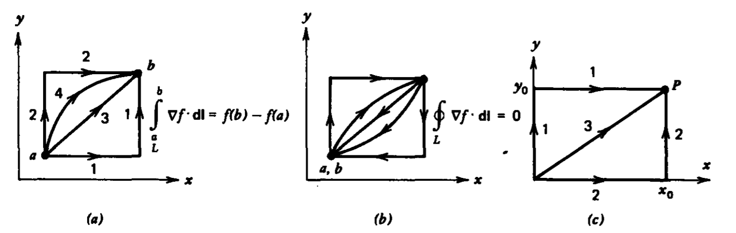
Figure 1-12b, then (15) is zero:

\[\oint_{L} \nabla f \cdot \textbf{dl} = f_{\vert_{a}} - f_{\vert_{a}} = 0 \]

where we indicate that the path is closed by the small circle in the integral sign f. The line integral of the gradient of a function around a closed path is zero.

Example 1-5: Line Integral

For \(f = x^{2}y\), verify (15) for the paths shown in Figure 1-12c between the origin and the point P at (x₀, y₀).

Solution

The total change in f between 0 and P is

\(\int_{0}^{P} df = f_{\vert_{P}} -f_{\vert_{0}} = x^{2}_{0}y_{0}\)

From the line integral along path I we find

\(\int_{0}^{P} \nabla f \cdot \textbf{dl} = \int_{y=0 \\ x=0}^{y_{0}} {\underbrace{\frac{\partial f}{\partial y}}_{x^{2}}} \nearrow^{0} \: dy \int_{x = 0 \\ y = y_{0}}^{x_{0}} \: \underbrace{\frac{\partial f}{\partial x}}_{2xy} dx = x_{0}^{2}y_{0}\)

Similarly, along path 2 we also obtain

\(\int_{0}^{P} \nabla f \cdot \textbf{dl} = \int_{x=0 \\ y=0}^{x_{0}} \underbrace{\frac{\partial f}{\partial x}}_{2xy} \nearrow^{0} \: dx + \int_{y=0 \\ x=x_{0}}^{y_{0}} \: \underbrace{\frac{\partial f}{\partial y}}_{x^{2}} dy = x_{0}^{2}y_{0}\)

while along path 3 we must relate x and y along the straight line as

\(y = \frac{y_{0}}{x_{0}}x \Rightarrow dy = \frac{y_{0}}{x_{0}} dx\)

to yield

\(\int_{0}^{P} \nabla f \cdot \textbf{dl} = \int_{0}^{P} (\frac{\partial f}{\partial x} dx + \frac{\partial f}{\partial y} dy) = \int_{x=0}^{x_{0}} \frac{3 y_{0}x^{2}}{x_{0}} dx = x_{0}^{2}y_{0}\)