1.2: Vector Algebra

Scalars and Vectors

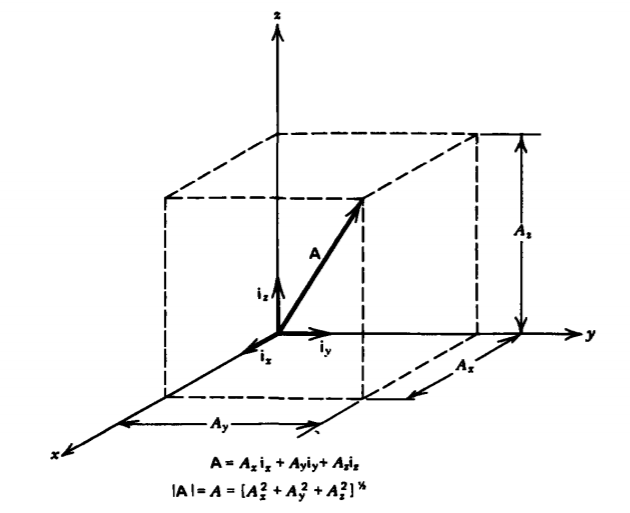
A scalar quantity is a number completely determined by its magnitude, such as temperature, mass, and charge, the last being especially important in our future study. Vectors, such as velocity and force, must-also have their direction specified and in this text are printed in boldface type. They are completely described by their components along three coordinate directions as shown for rectangular coordinates in Figure 1-4. A vector is represented by a directed line segment in the direction of the vector with its length proportional to its magnitude. The vector

\[\textbf{A} = A_{x}\textbf{i}_{x} + A_{y}\textbf{i}_{y} + A_{z}\textbf{i}_{z} \label{eq1} \]

in Figure 1-4 has magnitude

\[A = \mid A \mid = [A_{x}^{2} + A_{y}^{2} + A_{z}^{2}]^{1/2} \]

Note that each of the components in Equation \ref{eq1} (\(A_x\), \(A_y\), and \(A_z\)) are themselves scalars. The direction of each of the components is given by the unit vectors. We could describe a vector in any of the coordinate systems replacing the subscripts (x, y, z) by (r, \(\phi\), z) or (r, \(\theta\), \(\phi\)); however, for conciseness we often use rectangular coordinates for general discussion.

Figure 1-4 A vector is described by its components along the three coordinate directions.

Multiplication of a Vector by a Scalar

If a vector is multiplied by a positive scalar, its direction remains unchanged but its magnitude is multiplied by the scalar. If the scalar is negative, the direction of the vector is reversed:

\[a A = a A_{x} \textbf{i}_{x} + a A_{y} \textbf{i}_{y} + a A_{z} \textbf{i}_{x}  \]

Addition and Subtraction

The sum of two vectors is obtained by adding their components while their difference is obtained by subtracting their components. If the vector B

\[\textbf{B} = B_{x} \textbf{i}_{x} + B_{y}\textbf{i}_{y} + B_{z}\textbf{i}_{z}  \]

is added or subtracted to the vector A of Equation \ref{eq1}, the result is a new vector C:

\[\textbf{C} = \textbf{A} \pm \textbf{B} = (A_{x} \pm B_{x}) \textbf{i}_{x} + (A_{y} \pm B_{y})\textbf{i}_{y} + (A_{z} \pm B_{z})\textbf{i}_{z}  \]

Geometrically, the vector sum is obtained from the diagonal of the resulting parallelogram formed from A and B as shown in Figure 1-5a. The difference is found by first

Figure 1-5 The sum and difference of two vectors (a) by finding the diagonal of the parallelogram formed by the two vectors, and (b) by placing the tail of a vector at the head of the other.

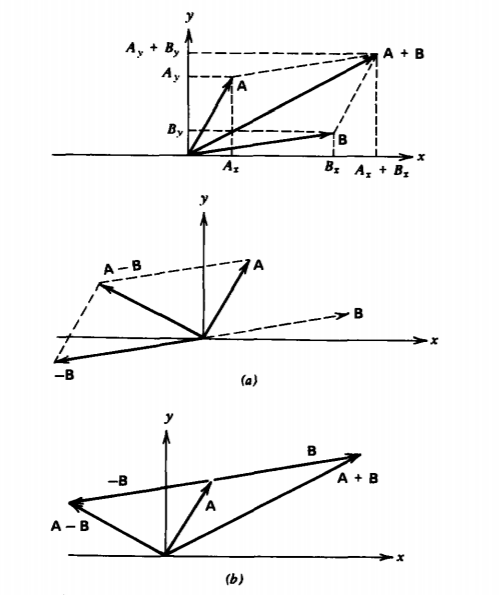
drawing -B and then finding the diagonal of the parallelogram formed from the sum of A and -B. The sum of the two vectors is equivalently found by placing the tail of a vector at the head of the other as in Figure 1-5b.

Subtraction is the same as addition of the negative of a vector.

Example 1-1: VECTOR ADDITION AND SUBTRACTION

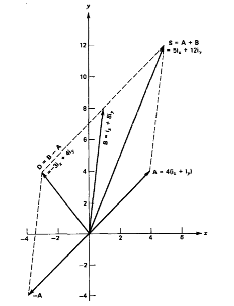
Given the vectors

\(\textbf{A} = 4\textbf{i}_{x} + 4 \textbf{i}_{y}, \: \: \textbf{B} = \textbf{i}_{x} + 8 \textbf{i}_{y}\)

find the vectors \(\textbf{B} \pm \textbf{A}\) and their magnitudes. For the geometric solution, see Figure 1-6.

Figure 1-6 The sum and difference of vectors A and B given in Example 1-1.

Solution

Sum

\(\textbf{S} = \textbf{A + B} = (4 +1)\textbf{i}_{x} + (4 + 8) \textbf{i}_{y} = 5 \textbf{i}_{x} + 12 \textbf{i}_{y}\)

\(S = [5^{2} + 12^{2}]^{1/2} = 13\)

Difference

\(\textbf{D=B-A} = (1-4) \textbf{i}_{x} + (8-4) \textbf{i}_{y} = -3\textbf{i}_{x} + 4\textbf{i}_{y}\)

\(D = [(-3)^{2} + 4^{2}]^{1/2} = 5\)

Dot (Scalar) Product

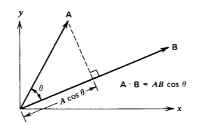
The dot product between two vectors results in a scalar and is defined as

\[\textbf{A} \cdot \textbf{B} = AB \: \cos \: \theta  \]

where \(\theta\) is the smaller angle between the two vectors. The term A cos \(\theta\) is the component of the vector A in the direction of B shown in Figure 1-7. One application of the dot product arises in computing the incremental work dW necessary to move an object a differential vector distance dl by a force F. Only the component of force in the direction of displacement contributes to the work

\[dW = \textbf{F} \cdot \textbf{dl}  \]

The dot product has maximum value when the two vectors are colinear (\(\theta\) =0) so that the dot product of a vector with itself is just the square of its magnitude. The dot product is zero if the vectors are perpendicular (\(\theta = \pi/2\)). These properties mean that the dot product between different orthogonal unit vectors at the same point is zero, while the dot

Figure 1-7 The dot product between two vectors.

product between a unit vector and itself is unity

\[\begin{matrix} \textbf{i}_{x} \cdot \textbf{i}_{x} = 1, & \textbf{i}_{x} \cdot \textbf{i}_{y} = 0 \\ \textbf{i}_{y} \cdot \textbf{i}_{y} = 1, & \textbf{i}_{x} \cdot \textbf{i}_{z} = 0 \\ \textbf{i}_{z} \cdot \textbf{i}_{z} = 1, & \textbf{i}_{y} \cdot \textbf{i}_{z} = 0 \end{matrix}  \]

Then the dot product can also be written as

\[\textbf{A} \cdot \textbf{B} = (A_{x} \textbf{i}_{x} + A_{y}\textbf{i}_{x} + A_{y}\textbf{i}_{y} + A_{z} \textbf{i}_{z}) \cdot (B_{x}\textbf{i}_{x} + B_{y}\textbf{i}_{y} + B_{x}\textbf{i}_{z}) = A_{x}B_{x} + A_{y}B_{y} + A_{z}B_{z}  \]

From (6) and (9) we see that the dot product does not depend on the order of the vectors

\[\textbf{A} \cdot \textbf{B = B} \cdot \textbf{A} \]

By equating (6) to (9) we can find the angle between vectors as

\[\cos \: \theta = \frac{A_{x}B_{x} + A_{y}B_{y} + A_{z}B_{z}}{AB}  \]

Similar relations to (8) also hold in cylindrical and spherical coordinates if we replace (x, y, z) by (r, \(\phi\), z) or (r, \(\theta\), \(\phi\)). Then (9) to (11) are also true with these coordinate substitutions.

Example 1-2: Dot Product

Find the angle between the vectors shown in Figure 1-8

\(\textbf{A} = \sqrt{3} \textbf{i}_{x} + \textbf{i}_{y}, \: \: \: \textbf{B} = 2 \textbf{i}_{x}\)

Figure 1-8 The angle between the two vectors A and B in Example 1-2 can be found using the dot product.

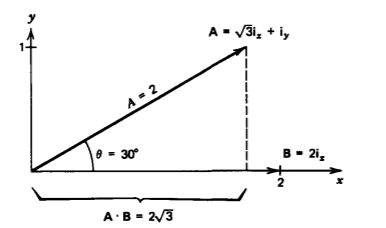
Solution

From (11)

\(\cos \: \theta = \frac{A_{x}B_{x}}{[A_{x}^{2} + A_{y}^{2}]^{1/2}B_{x}} = \frac{\sqrt{3}}{2}\)

\(\theta = \cos^{-1} \frac{\sqrt{3}}{2} = 30^{\circ}\)

Cross (Vector) Product

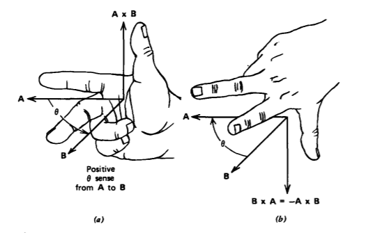
The cross product between two vectors A x B is defined as a vector perpendicular to both A and B, which is in the direction of the thumb when using the right-hand rule of curling the fingers of the right hand from A to B as shown in Figure 1-9. The magnitude of the cross product is

\[\vert \textbf{A} \times \textbf{B} \vert = AB \: \sin \: \theta  \]

where \(\theta\) is the enclosed angle between A and B. Geometrically, (12) gives the area of the parallelogram formed with A and B as adjacent sides. Interchanging the order of A and B reverses the sign of the cross product:

\[\textbf{A} \times \textbf{B} = - \textbf{B} \times \textbf{A}  \]

Figure 1-9 (a) The cross product between two vectors results in a vector perpendicular to both vectors in the direction given by the right-hand rule. (b) Changing the order of vectors in the cross product reverses the direction of the resultant vector.

The cross product is zero for colinear vectors (\(\theta\) =0) so that the cross product between a vector and itself is zero and is maximum for perpendicular vectors (\(\theta = \pi/2\)). For rectangular unit vectors we have

\begin{array}{lll}
\mathbf{i}_x \times \mathbf{i}_x=0, & \mathbf{i}_x \times \mathbf{i}_y=\mathbf{i}_z, & \mathbf{i}_y \times \mathbf{i}_x=-\mathbf{i}_x \\
\mathbf{i}_y \times \mathbf{i}_y=0, & \mathbf{i}_y \times \mathbf{i}_z=\mathbf{i}_x, & \mathbf{i}_x \times \mathbf{i}_y=-\mathbf{i}_x \\
\mathbf{i}_z \times \mathbf{i}_z=0, & \mathbf{i}_z \times \mathbf{i}_x=\mathbf{i}_y, & \mathbf{i}_x \times \mathbf{i}_x=-\mathbf{i}_y
\end{array}

These relations allow us to simply define a right-handed coordinate system as one where

\[\textbf{i}_{x} \times \textbf{i}_{y} = \textbf{i}_{z}  \]

Similarly, for cylindrical and spherical coordinates, righthanded coordinate systems have

\[\textbf{i}_{r} \times \textbf{i}_{\phi} = \textbf{i}_{z}, \: \: \: \textbf{i}_{r} \times \textbf{i}_{\theta} = \textbf{i}_{\phi}  \]

The relations of (14) allow us to write the cross product between A and B as

\[\textbf{A} \times \textbf{B} = (A_{x} \textbf{i}_{x} + A_{y}\textbf{i}_{y} + A_{z} \textbf{i}_{z}) \times (B_{x}\textbf{i}_{x} + B_{y}\textbf{i}_{y} + B_{z}\textbf{i}_{z}) = \textbf{i}_{x}(A_{y}B_{z}-A_{z}B_{y}) + \textbf{i}_{y}(A_{z}B_{x} - A_{x}B_{z}) + \textbf{i}_{z}(A_{x}B_{y}-A_{y}B_{x}) r \]

which can be compactly expressed as the determinantal expansion

\[\textbf{A} \times \textbf{B} = \det \begin{vmatrix} \textbf{i}_{x} & \textbf{i}_{y} & \textbf{i}_{z} \\ A_{x} & A_{y} & A_{z} \\ B_{x} & B_{y} & B_{z} \end{vmatrix} \\ = \textbf{i}_{x}(A_{y}B_{z} -A_{z}B_{y}) + \textbf{i}_{y}(A_{z}B_{x} - A_{x}B_{z}) + \textbf{i}_{z}(A_{x}B_{y} - A_{y}B_{x})  \]

The cyclical and orderly permutation of (x, y, z) allows easy recall of (17) and (18). If we think of xyz as a three-day week where the last day z is followed by the first day x, the days progress as

\[\underline{x \: y \: z} \: x \: \underline{y \: z \: x} \: y \: \underline {z \: x \: y} \: z \: ...  \]

where the three possible positive permutations are underlined. Such permutations of xyz in the subscripts of (18) have positive coefficients while the odd permutations, where xyz do not follow sequentially

\[xzy, \: yxz, \: zyx  \]

have negative coefficients in the cross product.

In (14)-(20) we used Cartesian coordinates, but the results remain unchanged if we sequentially replace (x, y, z) by the cylindrical coordinates (r, \(\theta\), z) or the spherical coordinates (r, \(\theta\), \(\phi\)).

Example 1-3: Cross Product

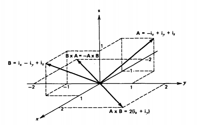
Find the unit vector i_n, perpendicular in the right-hand sense to the vectors shown in Figure 1-10.

\(\textbf{A} = - \textbf{i}_{x} + \textbf{i}_{y} + \textbf{i}_{z}, \: \: \textbf{B} = \textbf{i}_{x} - \textbf{i}_{y} + \textbf{i}_{z}\)

What is the angle between A and B?

Solution

The cross product A x B is perpendicular to both A and B

\(\textbf{A} \times \textbf{B} = \det \begin{vmatrix} \textbf{i}_{x} & \textbf{i}_{y} & \textbf{i}_{z} \\ -1 & 1 & 1 \\ 1 & -1 & 1 \end{vmatrix} = 2(\textbf{i}_{x} + \textbf{i}_{y})\)

The unit vector i_n is in this direction but it must have a magnitude of unity

\(\textbf{i}_{n} = \frac{\textbf{A} \times \textbf{B}}{\vert \textbf{A} \times \textbf{B} \vert} = \frac{1}{\sqrt{2}}(\textbf{i}_{x} + \textbf{i}_{y})\)

Figure 1-10 The cross product between the two vectors in Example 1-3.

The angle between A and B is found using (12) as

\(\sin \: \theta = \frac{\vert{\textbf{A} \times \textbf{B}}{AB} = \frac{2 \sqrt{2}}{\sqrt{3}\sqrt{3}} \\ = \frac{2}{3} \sqrt{2} \Rightarrow \theta = 70.5^{\circ} \textrm{ or } 109.5^{\circ}\)

The ambiguity in solutions can be resolved by using the dot product of (11)

\(\cos \: \theta = \frac{\textbf{A} \cdot \textbf{B}}{AB} = \frac{-1}{\sqrt{3}\sqrt{3}} = = \frac{1}{3} \Rightarrow \theta = 109.5^{\circ}\)