1.5: The Curl and Stokes' Theorem

Curl

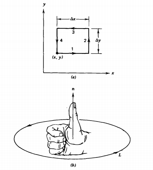
We have used the example of work a few times previously to motivate particular vector and integral relations. Let us do so once again by considering the line integral of a vector around a closed path called the circulation:

\[C = \oint_{L} \textbf{A} \cdot \textbf{dl} \]

where if \(C\) is the work, A would be the force. We evaluate (1) for the infinitesimal rectangular contour in Figure 1-19a:

\[C = \int_{x \\ 1}^{x + \Delta x} A_{x}(y) dx + \int_{y\\2}^{y + \Delta y} A_{y}(x + \Delta x) dy + \int_{x + \Delta x \\ 3}^{x} A_{x}(y+ \Delta y) dx + \int_{y + \Delta y \\ 4}^{y} A_{y}(x)dy \]

The components of A are approximately constant over each differential sized contour leg so that (2) is approximated as

\[C \approx \left(\dfrac{[A_{x}(y)-A_{x}(y + \Delta y)]}{\Delta y} + \dfrac{[A_{y}(x + \Delta x) - A_{y}(x)]}{\Delta x}\right) \Delta x \Delta y \]

where terms are factored so that in the limit as \(\Delta x\) and \(\Delta y\) become infinitesimally small, (3) becomes exact and the bracketed terms define partial derivatives:

\[\lim_{\Delta x \rightarrow 0 \\ \Delta y \rightarrow 0 \\ \Delta S_{z} = \Delta x \Delta y} \: C = (\dfrac{\partial A_{y}}{\partial x} - \dfrac{\partial A_{x}}{\partial y}) \Delta S_{z} \]

Figure 1-19 (a) Infinitesimal rectangular contour used to define the circulation. (b) The right-hand rule determines the positive direction perpendicular to a contour.

The contour in Figure 1-19a could just have as easily been in the xz or yz planes where (4) would equivalently become

\[C = (\dfrac{\partial A_{z}}{\partial y} - \dfrac{\partial A_{y}}{\partial z}) \Delta S_{x} \: \: (yz \textrm{ plane}) \\ C = (\dfrac{\partial A_{x}}{\partial z} - \dfrac{\partial A_{z}}{\partial x}) \Delta S_{y} \: \: (xz \textrm{ plane}) \]

by simple positive permutations of x, y, and z.

The partial derivatives in (4) and (5) are just components of the cross product between the vector del operator of Section 1-3-1 and the vector A. This operation is called the curl of A and it is also a vector:

\[\textrm{curl} \textbf{ A} = \nabla \times \textbf{A} = \textrm{det} \begin{vmatrix} \textbf{i}_{x} & \textbf{i}_{y} & \textbf{i}_{z} \\ \dfrac{\partial}{\partial x} & \dfrac{\partial}{\partial y} & \dfrac{\partial}{\partial z} \\ A_{x} & A_{y} & A_{z} \end{vmatrix} \\ = \textbf{i}_{x}(\dfrac{\partial A_{z}}{\partial y} - \dfrac{\partial A_{y}}{\partial z}) + \textbf{i}_{y}(\dfrac{\partial A_{x}}{\partial z} - \dfrac{\partial A_{z}}{\partial x}) + \textbf{i}_{z}(\dfrac{\partial A_{y}}{\partial x} - \dfrac{\partial A_{x}}{\partial y}) \]

The cyclical permutation of (x, y, z) allows easy recall of (6) as described in Section 1-2-5.

In terms of the curl operation, the circulation for any differential sized contour can be compactly written as

\[C = (\nabla \times \textbf{A}) \cdot \textbf{dS} \]

where dS = n dS is the area element in the direction of the normal vector n perpendicular to the plane of the contour in the sense given by the right-hand rule in traversing the contour, illustrated in Figure 1-19b. Curling the fingers on the right hand in the direction of traversal around the contour puts the thumb in the direction of the normal n.

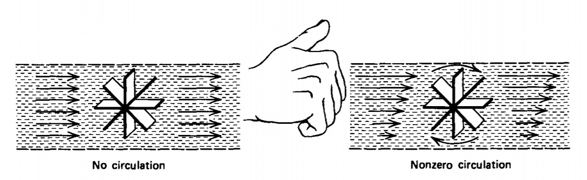
For a physical interpretation of the curl it is convenient to continue to use a fluid velocity field as a model although the general results and theorems are valid for any vector field. If a small paddle wheel is imagined to be placed without disturbance in a fluid flow, the velocity field is said to have circulation, that is, a nonzero curl, if the paddle wheel rotates as illustrated in Figure 1-20. The curl component found is in the direction of the axis of the paddle wheel.

Figure 1-20 A fluid with a velocity field that has a curl tends to turn the paddle wheel. The curl component found is in the same direction as the thumb when the fingers of the right hand are curled in the direction of rotation.

Curl for Curvilinear Coordinates

A coordinate independent definition of the curl is obtained using (7) in (1) as

\[(\nabla \times \textbf{A})_{n} = \lim_{dS_{n} \rightarrow 0} \dfrac{\oint_{L} \textbf{A} \cdot \textbf{dl}}{dS_{n}} \]

where the subscript n indicates the component of the curl perpendicular to the contour. The derivation of the curl operation (8) in cylindrical and spherical. coordinates is straightforward but lengthy.

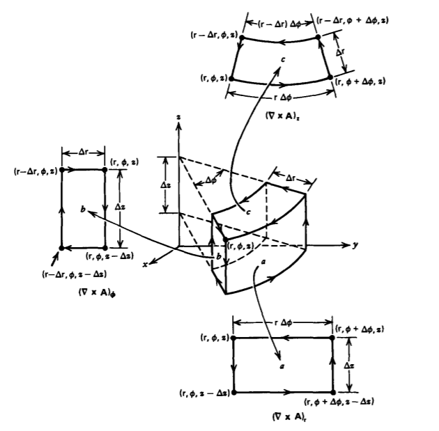
(a) Cylindrical Coordinates To express each of the components of the curl in cylindrical coordinates, we use the three orthogonal contours in Figure 1-21. We evaluate the line integral around contour a:

\[\oint_{a} \textbf{A} \cdot \textbf{dl} = \int_{z}^{z - \Delta z} A_{z}(\phi) dz + \int_{\phi}^{\phi + \Delta \phi} A_{\phi} (z - \Delta z) \textrm{r} \: d \phi \\ + \int_{z - \Delta z}^{z} A_{z} (\phi + \Delta \phi) dz + \int_{\phi + \Delta \phi}^{\phi} A_{\phi} (z) \textrm{r} \: d \phi \\ \approx (\dfrac{[A_{z} (\phi + \Delta \phi) - A_{z} (\phi)]}{\textrm{r} \Delta \phi} - \dfrac{[A_{\phi}(z) - A_{\phi}(z - \Delta z)]}{\Delta z}) \textrm{r} \: \Delta \phi \: \Delta z \]

Figure 1-21 Incremental contours along cylindrical surface area elements used to calculate each component of the curl of a vector in cylindrical coordinates.

to find the radial component of the curl as

\[(\nabla \times \textbf{A})_{\textrm{r}} = \lim_{\Delta \phi \rightarrow 0 \\ \Delta z \rightarrow 0} \dfrac{\oint_{a} \textbf{A} \cdot \textbf{dl}}{\textrm{r} \: \Delta \phi \: \Delta z} = \dfrac{1}{\textrm{r}} \dfrac{\partial A_{z}}{\partial \phi} - \dfrac{\partial A_{\phi}}{\partial z} \]

We evaluate the line integral around contour b

\[\oint_{b} \textbf{A} \cdot \textbf{dl} = \int_{r-\Delta r}^{r} A_{\textrm{r}}(z) d \textrm{r} + \int_{z}^{z - \Delta z} A_{z}(\textrm{r})dz + \int_{\textrm{r}}^{\textrm{r} - \Delta \textrm{r}} A_{\textrm{r}}(z- \Delta z) d \textrm{r} + \int_{z - \Delta z}^{z} A_{z}(\textrm{r}-\Delta \textrm{r}) dz \\ \approx (\dfrac{[A_{\textrm{r}}(z) - A_{\textrm{r}}(z-\Delta z)]}{\Delta z} - \dfrac{[A_{z}(\textrm{r}) - A_{z}(\textrm{r}- \Delta \textrm{r})]}{\Delta \textrm{r}}) \Delta \textrm{r} \Delta z \]

to find the \(\phi\) component of the curl,

\[(\nabla \times \textbf{A})_{\phi} = \lim_{\Delta \textrm{r} \rightarrow 0 \\ \Delta z \rightarrow 0} \dfrac{\oint_{b} \textbf{A} \cdot \textbf{dl}}{\Delta \textrm{r} \Delta z} = (\dfrac{\partial A_{\textrm{r}}}{\partial z} - \dfrac{\partial A_{z}}{\partial \textrm{r}}) \]

The z component of the curl is found using contour c:

\[\oint_{c} \textbf{A} \cdot \textbf{dl} = \int_{\textrm{r} - \Delta \textrm{r}}^{\textrm{r}} A_{\textrm{r}_{\mid \phi}} d \textrm{r} + \int_{\phi}^{\phi + \Delta \phi} \textrm{r} A_{\phi_{\mid \textrm{r}}} d \phi + \int_{\textrm{r}}^{\textrm{r}- \Delta \textrm{r}} A_{\textrm{r}_{\mid \phi + \Delta \phi}} d \textrm{r} \\ + \int_{\phi + \Delta \phi}^{\phi} (\textrm{r} - \Delta \textrm{r}) A_{\phi_{\mid \textrm{r} - \Delta \textrm{r}}} d \phi \\ \approx (\dfrac{[\textrm{r}A_{\phi_{\mid \textrm{r}}} - (\textrm{r} - \Delta \textrm{r}) A_{\phi_{\mid \textrm{r} - \Delta \textrm{r}}}]}{\textrm{r} \Delta \textrm{r}} - \dfrac{[A_{\textrm{r}_{\mid \phi + \Delta \phi}} - A_{\textrm{r}_{\mid \phi}}]}{\textrm{r} \Delta \phi}) \textrm{r} \Delta \textrm{r} \Delta \phi \]

to yield

\[(\nabla \times \textbf{A})_{z} = \lim_{\Delta \textrm{r} \rightarrow 0 \\ \Delta \phi \rightarrow 0} \dfrac{\oint_{c} \textbf{A} \cdot \textbf{dl}}{\textrm{r} \Delta \textrm{r} \Delta \phi} = \dfrac{1}{\textrm{r}} (\dfrac{\partial}{\partial \textrm{r}} (\textrm{r} A_{\phi}) - \dfrac{\partial A_{\textrm{r}}}{\partial \phi}) \]

The curl of a vector in cylindrical coordinates is thus

\[\nabla \times \textbf{A} = (\dfrac{1}{\textrm{r}} \dfrac{\partial A_{z}}{\partial \phi} - \dfrac{\partial A_{\phi}}{\partial z})\textbf{i}_{\textrm{r}} + (\dfrac{\partial A_{\textrm{r}}}{\partial z} - \dfrac{\partial A_{z}}{\partial \textrm{r}})\textbf{i}_{\phi} \\ + \dfrac{1}{\textrm{r}} (\dfrac{\partial}{\partial \textrm{r}} (\textrm{r} A_{\phi}) - \dfrac{\partial A_{\textrm{r}}}{\partial \phi})\textbf{i}_{z} \]

(b) Spherical Coordinates

Similar operations on the three incremental contours for the spherical element in Figure 1-22 give the curl in spherical coordinates. We use contour a for the radial component of the curl:

\[\oint_{a} \textbf{A} \cdot \textbf{dl} = \int_{\phi}^{\phi + \Delta \phi} A_{\phi_{\mid \theta}} r \: \sin \: \theta \: d \phi + \int_{\theta}^{\theta - \Delta \theta} r A_{\theta_{\mid \: \phi + \Delta \phi}} d \theta \\ + \int_{\phi + \Delta \phi}^{\phi} r \: \sin \: (\theta - \Delta \theta)A_{\phi_{\mid \theta - \Delta \theta}} d \phi + \int_{\theta - \Delta \theta}^{\theta} r A_{\theta_{\mid \phi}} d \theta \\ \approx (\dfrac{[A_{\phi_{\mid \theta}} \: \sin \: \theta - A_{\phi_{\mid \theta - \Delta \theta}} \: \sin \: (\theta - \Delta \theta)]}{r \: \sin \: \theta \: \Delta \theta} - \dfrac{[A_{\theta_{\mid \phi + \Delta \phi}} - A_{\theta_{\mid \phi}}]}{r \: \sin \: \theta \: \Delta \phi})r^{2} \: \sin \: \theta \: \Delta \theta \: \Delta \: \phi \]

to obtain

\[(\nabla \times \textbf{A})_{r} = \lim_{\Delta \theta \rightarrow 0 \\ \Delta \phi \rightarrow 0} \dfrac{\oint_{a} \textbf{A} \cdot \textbf{dl}}{r^{2} \: \sin \: \theta \: \Delta \theta \: \Delta \phi} = frac{1}{r \: \sin \: \theta}(\dfrac{\partial}{\partial \theta}(A_{\phi} \: \sin \: \theta)- \dfrac{\partial A_{\theta}}{\partial \phi}) \]

Figure 1-22 Incremental contours along spherical surface area elements used to calculate each component of the curl of a vector in spherical coordinates.

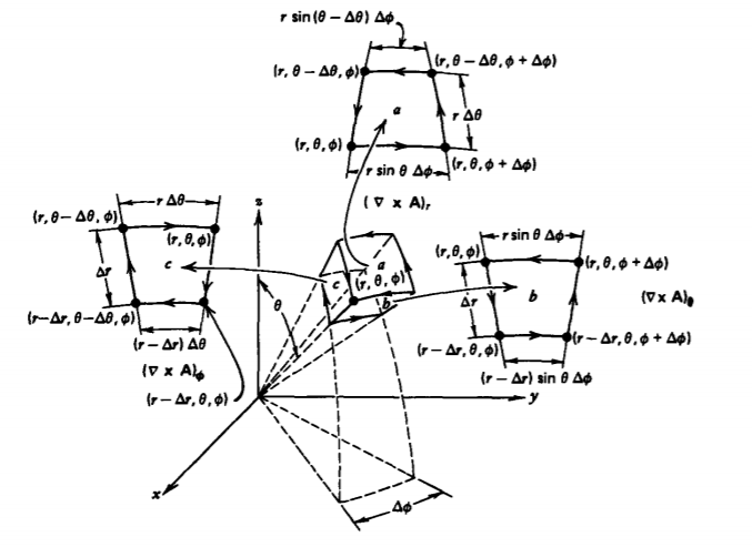
The \(\theta\) component is found using contour b:

\[\oint_{b} \textbf{A} \cdot \textbf{dl} = \int_{r}^{r- \Delta r} A_{r_{\mid \phi}} dr + \int_{\phi}^{\phi + \Delta \phi} (r - \Delta r) A_{\phi_{\mid r - \Delta r}} \: \sin \: \theta \: d \phi \\ + \int_{r - \Delta r}^{r} A_{r_{\mid \phi + \Delta phi}} dr + \int_{\phi + \Delta \phi}^{\phi} r A_{\phi_{\mid r}} \: \sin \: \theta \: d \phi \\ \approx (\dfrac{[A_{r_{\mid \phi + \Delta \phi}} - A_{r_{\mid \phi}}]}{r \: \sin \: \theta \: \Delta \phi} - \dfrac{[rA_{\phi_{\mid r}} - (r - \Delta r) A_{\phi_{\mid r - \Delta r}}]}{r \Delta r}) r \: \sin \: \theta \: \Delta r \: \Delta \phi \]

\[(\nabla \times A)_{\theta} = \lim_{\Delta r \rightarrow 0 \\ \Delta \phi \rightarrow 0} \dfrac{\oint_{b} \textbf{A} \cdot \textbf{dl}}{r \: \sin \: \theta \: \Delta r \: \Delta \phi} = \dfrac{1}{r} (\dfrac{1}{\sin \: \theta}{\partial A_{r}}{\partial \phi} - \dfrac{\partial}{\partial r}(rA_{phi})) \]

The 4 component of the curl is found using contour c:

\[\oint_{c} \textbf{A} \cdot \textbf{dl} = \int_{\theta - \Delta \theta}^{\theta} rA_{\theta_{\mid r}} d \theta + \int_{r}^{r-\Delta r} A_{r_{\mid \theta}} dr \\ + \int_{\theta}^{\theta - \Delta \theta} (r- \Delta r) A_{\theta_{\mid r- \Delta r}} d \theta + \int_{r - \Delta r}^{r} A_{r_{\mid \theta - \Delta \theta}} dr \\ \approx (\dfrac{[r A_{\theta_{\mid r}} - (r - \Delta r) A_{\theta_{\mid r - \Delta r}}]}{r \Delta r} - \dfrac{[A_{r_{\mid \theta}} - A_{r_{\mid \theta - \Delta \theta}}]}{r \Delta \theta}) r \: \Delta r \: \Delta \theta \]

as

\[(\nabla \times \textbf{A})_{\phi} = \lim_{\Delta r \rightarrow 0 \\ \Delta \theta \rightarrow 0} \dfrac{\oint_{c} \textbf{A} \cdot \textbf{dl}}{r \: \Delta r \: \Delta \theta} = \dfrac{1}{r}(\dfrac{\partial}{\partial r} (r A_{\theta}) - \dfrac{\partial A_{r}}{\partial \theta}) \]

The curl of a vector in spherical coordinates is thus given from (17), (19), and (21) as

\[\nabla \times \textbf{A} = \dfrac{1}{r \: \sin \: \theta} (\dfrac{\partial}{\partial \theta} (A_{\phi} \: \sin \: \theta) - \dfrac{\partial A_{\theta}}{\partial \phi}) \textbf{i}_{r} \\ + \dfrac{1}{r}(\dfrac{1}{\sin \: \theta} \dfrac{\partial A_{r}}{\partial \phi} - \dfrac{\partial}{\partial r}(r A_{\phi}))\textbf{i}_{\theta} \\ + \dfrac{1}{r}(\dfrac{\partial}{\partial r} (r A_{\theta}) - \dfrac{\partial A_{r}}{\partial \theta})\textbf{i}_{\phi} \]

Stokes' Theorem

We now piece together many incremental line contours of the type used in Figures 1-19-1-21 to form a macroscopic surface S like those shown in Figure 1-23. Then each small contour generates a contribution to the circulation

\[dC = (\nabla \times \textbf{A}) \cdot \textbf{dS} \]

so that the total circulation is obtained by the sum of all the small surface elements

\[C = \int_{S} (\nabla \times \textbf{A}) \cdot \textbf{dS} \]

Figure 1-23 Many incremental line contours distributed over any surface, have nonzero contribution to the circulation only along those parts of the surface on the boundary contour \(L\).

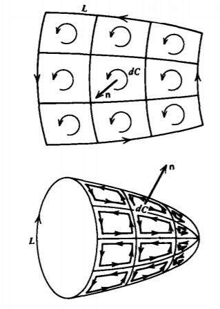
Each of the terms of (23) are equivalent to the line integral around each small contour. However, all interior contours share common sides with adjacent contours but which are twice traversed in opposite directions yielding no net line integral contribution, as illustrated in Figure 1-23. Only those contours with a side on the open boundary L have a nonzero contribution. The total result of adding the contributions for all the contours is Stokes' theorem, which converts the line integral over the bounding contour L of the outer edge to a surface integral over any area S bounded by the contour

\[\oint_{L} \textbf{A} \cdot \textbf{dl} = \int_{S}(\nabla \times \textbf{A}) \cdot \textbf{dS} \]

Note that there are an infinite number of surfaces that are bounded by the same contour \(L\). Stokes' theorem of (25) is satisfied for all these surfaces.

Example 1-7: STOKES' THEOREM

Verify Stokes' theorem of (25) for the circular bounding contour in the xy plane shown in Figure 1-24 with a vector

field

 

Check the result for the (a) flat circular surface in the xy plane, (b) for the hemispherical surface bounded by the contour, and (c) for the cylindrical surface bounded by the contour.

Figure 1-24 Stokes' theorem for the vector given in Example 1-7 can be applied to any surface that is bounded by the same contour L.

Solution

For the contour shown

\[\textbf{dl} = R \: d \phi : \textbf{i}_{\phi} \nonumber \]

so that

\[\textbf{A} \cdot \textbf{dl} = R^{2} d \phi \nonumber \]

where on L, r = R. Then the circulation is

\[C = \oint_{L} \textbf{A} \cdot \textbf{dl} = \int_{0}^{2 \pi} R^{2} \: d \phi = 2 \pi R^{2} \nonumber \]

The z component of A had no contribution because dl was entirely in the xy plane.

The curl of A is

\[\nabla \times \textbf{A} = \textbf{i}_{z}(\dfrac{\partial A_{y}}{\partial x} - \dfrac{\partial A_{x}}{\partial y}) = 2 \textbf{i}_{z} \nonumber \]

(a) For the circular area in the plane of the contour, we have that

\[\int_{S} (\nabla \times \textbf{A}) \cdot \textbf{dS} = 2 \int_{S} dS_{z} = 2 \pi R^{2} \nonumber \]

which agrees with the line integral result.

(b) For the hemispherical surface

\[\int_{S}(\nabla \times \textbf{A}) \cdot \textbf{dS} = \int_{\theta = 0}^{\pi/2} \int_{\phi=0}^{2 \pi} 2 \textbf{i}_{z} \cdot \textbf{i}_{r}R^{2} \: \sin \: \theta \: d \theta \: d \phi \nonumber \]

From Table 1-2 we use the dot product relation

\[\textbf{i}_{z} \cdot \textbf{i}_{r} = \cos \: \nonumber \theta \]

which again gives the circulation as

\[C = \int_{\theta = 0}^{\pi/2} \int_{\phi = 0}^{2 \pi} R^{2} \: \sin \: 2 \theta \: d \theta \: d \phi = -2 \pi R^{2} \dfrac{\cos 2 \theta}{2} \bigg|_{\theta = 0}^{\pi/2} = 2 \pi R^{2} \nonumber \]

(c) Similarly, for the cylindrical surface, we only obtain nonzero contributions to the surface integral at the upper circular area that is perpendicular to \(\nabla \times \textbf{A}\). The integral is then the same as part (a) as \(\nabla \times \textbf{A}\) is independent of z.

Some Useful Vector Identities

The curl, divergence, and gradient operations have some simple but useful properties that are used throughout the text.

(a) The Curl of the Gradient is Zero

\[\nabla \times (\nabla f)= 0 \]

We integrate the normal component of the vector \(\nabla \times (\nabla f)\) over a surface and use Stokes' theorem

\[\int_{s} \nabla \times (\nabla f) \cdot \textbf{dS} = \oint_{L} \nabla f \cdot \textbf{dl} = 0 \]

where the zero result is obtained from Section 1-3-3, that the line integral of the gradient of a function around a closed path is zero. Since the equality is true for any surface, the vector coefficient of dS in (26) must be zero

\[\nabla \times (\nabla f) = 0 \nonumber \]

The identity is also easily proved by direct computation using the determinantal relation in Section 1-5-1 defining the curl operation:

\[\begin{align*} \nabla \times (\nabla f) &= \det \begin{vmatrix} \textbf{i}_{x} & \textbf{i}_{y} & \textbf{i}_{z} \\ \dfrac{\partial}{\partial x} & \dfrac{\partial}{\partial y} & \dfrac{\partial}{\partial z} \\ \dfrac{\partial f}{\partial x} & \dfrac{\partial f}{\partial y} & \dfrac{\partial f}{\partial z} \end{vmatrix} \\[4pt] &= \textbf{i}_{x} \left(\dfrac{\partial^{2}f}{\partial y \partial z} - \dfrac{\partial^{2} f}{\partial z \partial y}\right) + \textbf{i}_{y} \left(\dfrac{\partial^{2}f}{\partial z \partial x} - \dfrac{\partial ^{2} f}{\partial x \partial x}\right) + \textbf{i}_{z}\left(\dfrac{\partial^{2}f}{\partial x \partial y} - \dfrac{\partial^{2}f}{\partial y \partial x}\right) \\[4pt] &= 0 \end{align*} \]

Each bracketed term in (28) is zero because the order of differentiation does not matter.

(b) The Divergence of the Curl of a Vector is Zero

\[\nabla - (\nabla \times \textbf{A}) = 0 \]

One might be tempted to apply the divergence theorem to the surface integral in Stokes' theorem of (25). However, the divergence theorem requires a closed surface while Stokes' theorem is true in general for an open surface. Stokes' theorem for a closed surface requires the contour \(L\) to shrink to zero giving a zero result for the line integral. The divergence theorem applied to the closed surface with vector \(\nabla \times \textbf{A}\) is then

\[\oint_{S} \nabla \times \textbf{A} \cdot \textbf{dS} = 0 \Rightarrow \int_{V} \nabla \cdot (\nabla \times \textbf{A}) dV = 0 \Rightarrow \nabla \cdot (\nabla \times \textbf{A}) = 0 \]

which proves the identity because the volume is arbitrary.

More directly we can perform the required differentiations

\[\begin{align} \nabla \cdot (\nabla \times \textbf{A}) &= \dfrac{\partial}{\partial x}\left (\dfrac{\partial A_{z}}{\partial y} - \dfrac{\partial A_{y}}{\partial z}\right) + \dfrac{\partial}{\partial y} \left(\dfrac{\partial A_{x}}{\partial z} - \dfrac{\partial A_{z}}{\partial x}\right) + \dfrac{\partial}{\partial z} \left(\dfrac{\partial A_{y}}{\partial x} - \dfrac{\partial A_{x}}{\partial y}\right) \nonumber \\[4pt] &= \left(\dfrac{\partial^{2} A_{z}}{\partial x \partial y} - \dfrac{\partial^{2} A_{z}}{\partial y \partial x}\right) + \left(\dfrac{\partial^{2}A_{x}}{\partial y \partial z} - \dfrac{\partial^{2}A_{x}}{\partial z \partial y}\right) + \left(\dfrac{\partial^{2}A_{y}}{\partial z \partial x} - \dfrac{\partial^{2}A_{y}}{\partial x \partial z}\right) \nonumber \\[4pt] &= 0 \end{align} \]

where again the order of differentiation does not matter.