2.3: Charge Distributions

The method of superposition used in Section 2.2.4 will be used throughout the text in relating fields to their sources. We first find the field due to a single-point source. Because the field equations are linear, the net field due to many point sources is just the superposition of the fields from each source alone. Thus, knowing the electric field for a single-point charge-at an arbitrary position immediately gives us the total field for any distribution of point charges.

In typical situations, one coulomb of total charge may be present requiring 6.25 x 10¹⁸ elementary charges (e ≈1.60 x 10^-19 coul). When dealing with such a large number of particles, the discrete nature of the charges is often not important and we can consider them as a continuum. We can then describe the charge distribution by its density. The same model is used in the classical treatment of matter. When we talk about mass we do not go to the molecular scale and count the number of molecules, but describe the material by its mass density that is the product of the local average number of molecules in a unit volume and the mass per molecule.

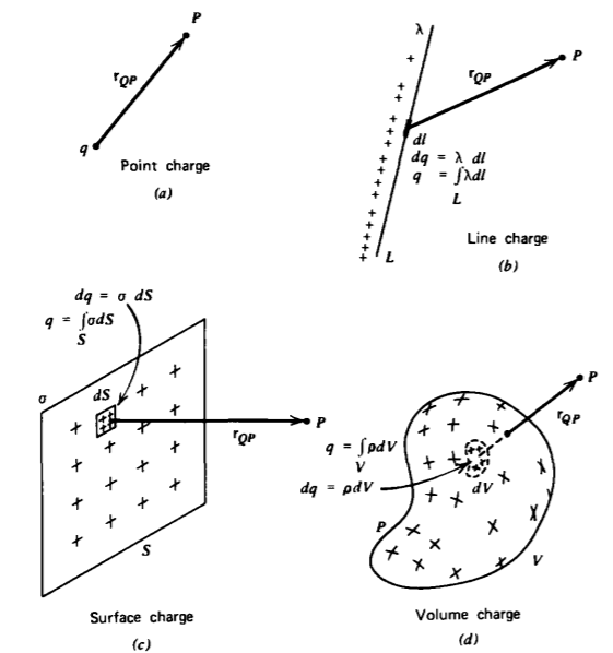
Line, Surface, and Volume Charge Distributions

We similarly speak of charge densities. Charges can distribute themselves on a line with line charge density \(\lambda\) (coul/m), on a surface with surface charge density \(\sigma\) (coul/m²) or throughout a volume with volume charge density \(\rho\) (coul/m³)

Consider a distribution of free charge dq of differential size within a macroscopic distribution of line, surface, or volume charge as shown in Figure 2-9. Then, the total charge q within each distribution is obtained by summing up all the differential elements. This requires an integration over the line, surface, or volume occupied by the charge.

\[dq = \left\{ \begin{array}{ll} \lambda dl \\ \sigma \: dS \Rightarrow q = \\ \rho \: d V \end{array} \right. \left \{ \begin{array}{ll} \int_{l} \lambda \: dl \: \textrm{(line charge)} \\ \int_{S} \sigma \: dS \: \textrm{(surface charge)} \\ \int_{V} \rho \: dV \: \textrm{(volume charge)} \end{array} \right. \]

Example 2-2: Charge Distribution

Find the total charge within each of the following distributions illustrated in Figure 2-10

(a) Line charge \(\lambda_{0}\) uniformly distributed in a circular hoop of radius a.

Figure 2-9 Charge distributions. (a) Point charge; (b) Line charge; (c) Surface charge; (d) Volume charge.

(b) Surface charge \(\sigma_{0}\) uniformly distributed on a circular disk of radius a.

(c) Volume charge \(\rho_{0}\) uniformly distributed throughout a sphere of radius R.

Figure 2-10 Charge distributions of Example 2-2. (a) Uniformly distributed line charge on a circular hoop. (b) Uniformly distributed surface charge on a circular disk. (c) Uniformly distributed volume charge throughout a sphere. (d) Nonuniform line charge distribution. (e) Smooth radially dependent volume charge distribution throughout all space, as a simple model of the electron cloud around the positively charged nucleus of the hydrogen atom.

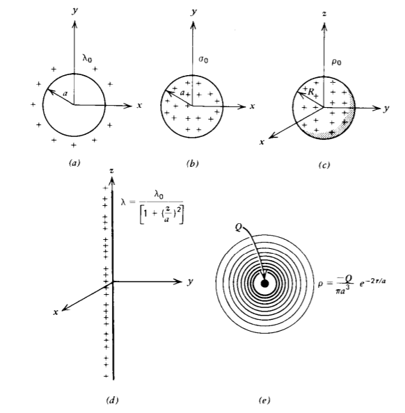
(d) A line charge of infinite extent in the z direction with charge density distribution

\(\lambda = \frac{\lambda_{0}}{[1 + (z/a)^{2}]}\)

(e) The electron cloud around the positively charged nucleus Q in the hydrogen atom is simply modeled as the spherically symmetric distribution

\(\rho(r) = \frac{Q}{\pi a^{3}} e^{-2r/a}\)

Solution

(a) \(q = \int_{L} \lambda \: dl = \int_{0}^{2 \pi} \lambda_{0}a \: d \phi = 2 \pi a \lambda_{0}\)

(b) \(q = \int_{S} \sigma d \textrm{S} = \int_{\textrm{r} = 0}^{2 \pi} \sigma_{0} \textrm{r} d \textrm{r} \: d \pi a^{2} \sigma_{0}\)

(c) \(q = \int_{V} \rho \: dV = \int_{r = 0}^{R} \int_{\theta = 0}^{\pi} \int_{\phi 0}^{2 \pi} \rho_{0}r^{2} \sin \: \theta dr \: d \theta \: d \phi = \frac{4}{3} \pi R^{3} \rho_{0}\)

(d) \(q = \int_{L} \lambda \: dl = \int_{- \infty}^{+ \infty} \frac{\lambda_{0} dz}{[1 + (z/a)^{2}]} = \lambda_{0}a \: \tan^{-1} \frac{z}{a} \bigg|_{- \infty}^{+ \infty} = \lambda_{0}\pi a\)

The total charge in the cloud is

\(q = \int_{V} \rho \: dV \\ = -\int_{r = 0}^{\infty} \int_{\theta = 0}^{\pi} \int_{\phi = 0}^{2 \pi} \frac{Q}{\pi a^{3}} e^{-2r/a} r^{2} \sin \: \theta \: dr \: d \theta \: d \phi \\ = -\int_{r = 0}^{\infty} \frac{4Q}{a^{3}}e^{-2r/a} r^{2} \: dr \\ = -\frac{4Q}{a^{3}} (- \frac{a}{2}) e^{-2r/a} [r^{2} - \frac{a^{2}}{2}(-\frac{2r}{a} -1)] \bigg|_{r = 0}^{\infty} \\ = -Q\)

Electric Field Due to a Charge Distribution

Each differential charge element dq as a source at point Q contributes to the electric field at. a point P as

\[d \textbf{E} = \frac{dq}{4 \pi \varepsilon_{0} r^{2}_{QP}} \textbf{i}_{QP} \]

where r_QP is the distance between Q and P with i_QP the unit vector directed from Q to P. To find the total electric field, it is necessary to sum up the contributions from each charge element. This is equivalent to integrating (2) over the entire charge distribution, remembering that both the distance r_QP and direction i_QP vary for each differential element throughout the distribution

\[\textbf{E} = \int_{\textbf{all} \: q} \frac{dq}{4 \pi \varepsilon_{0}r_{QP}^{2}} \textbf{i}_{QP} \]

where (3) is a line integral for line charges (\(dq = \lambda \: dl\)), a surface integral for surface charges (\(dq = \sigma \: dS\)), a volume integral for a volume charge distribution (\(dq = \rho \: dV\)), or in general, a combination of all three.

If the total charge distribution is known, the electric field is obtained by performing the integration of (3). Some general rules and hints in using (3) are:

1. It is necessary to distinguish between the coordinates of the field points and the charge source points. Always integrate over the coordinates of the charges.
2. Equation (3) is a vector equation and so generally has three components requiring three integrations. Symmetry arguments can often be used to show that particular field components are zero.
3. The distance r_QP is always positive. In taking square roots, always make sure that the positive square root is taken.
4. The solution to a particular problem can often be obtained by integrating the contributions from simpler differential size structures.

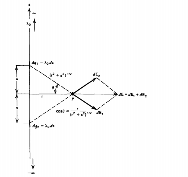
Field Due to an Infinitely Long Line Charge

An infinitely long uniformly distributed line charge \(\lambda_{0}\) along the z axis is shown in Figure 2-11. Consider the two symmetrically located charge elements dq₁ and dq₂ a distance z above and below the point P, a radial distance r away. Each charge element alone contributes radial and z components to the electric field. However, just as we found in Example 2-1a, the two charge elements together cause equal magnitude but oppositely directed z field components that thus cancel leaving only additive radial components:

\[dE_{\textrm{r}} = \frac{\lambda_{0} dz}{4 \pi \epsilon_{0}(z^{2} + \textrm{r}^{2})} \cos \: \theta = \frac{\lambda_{0} \textrm{r} dz}{4 \pi \varepsilon_{0}(z^{2} + \textrm{r}^{2})^{3/2}} \]

To find the total electric field we integrate over the length of the line charge:

\[E_{\textrm{r}} = \frac{\lambda_{0} \textrm{r}}{4 \pi \varepsilon_{0}} \int_{- \infty}^{+ \infty} \frac{dz}{(z^{2} + \textrm{r}^{2})^{3/2}} \\ = \frac{\lambda_{0} \textrm{r}}{4 \pi \varepsilon_{0}} \frac{z}{\textrm{r}^{2}(z^{2} + \textrm{r}^{2})^{1/2}} \bigg|_{z = - \infty}^{+ \infty} \\ = \frac{\lambda_{0}}{2 \pi \varepsilon_{0} \textrm{r}} \]

Figure 2-8a.

Field Due to Infinite Sheets of Surface Charge

(a) Single Sheet

A surface charge sheet of infinite extent in the y =0 plane has a uniform surface charge density \(\sigma_{0}\) as in Figure 2-12a. We break the sheet into many incremental line charges of thickness dx with \(d \lambda = \sigma_{0} dx\). We could equivalently break the surface into incremental horizontal line charges of thickness dz. Each incremental line charge alone has a radial field component as given by (5) that in Cartesian coordinates results in x and y components. Consider the line charge \(d \lambda_{1}\), a distance x to the left of P, and the symmetrically placed line charge \(d \lambda_{2}\) the same distance x to the right of P. The x components of the resultant fields cancel while the y

Figure 2-12 (a) The electric field from a uniformly surface charged sheet of infinite extent is found by summing the contributions from each incremental line charge element. Symmetrically placed line charge elements have x field components that cancel, but y field components that add. (b) Two parallel but oppositely charged sheets of surface charge have fields that add in the region between the sheets but cancel outside. (c) The electric field from a volume charge distribution is obtained by summing the contributions from each incremental surface charge element

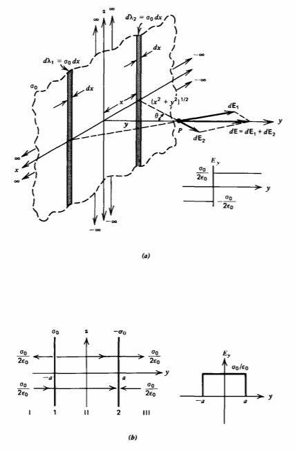
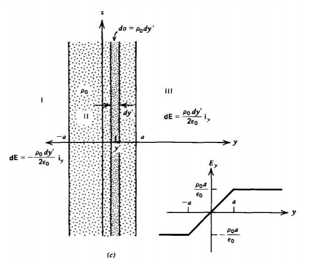
Fig. 2-12(c)

components add:

\[dE_{y} = \frac{\sigma_{0}dx}{2 \pi \varepsilon_{0}(x^{2} + y^{2})^{1/2}} \cos \: \theta = \frac{\sigma_{0}y \: dx}{2 \pi \varepsilon_{0}(x^{2} + y^{2})} \]

The total field is then obtained by integration over all line charge elements:

\[E_{y} = \frac{\sigma_{0}y}{2 \pi \varepsilon_{0}} \int_{- \infty}^{+ \infty} \frac{dx}{x^{2} + y^{2}} \\ \frac{\sigma_{0}y}{2 \pi \varepsilon_{0}} \frac{1}{y} \tan^{-1} \frac{x}{y} \bigg|_{x = - \infty}^{+ \infty} \\ = \left \{ \begin{matrix} \sigma_{0}/2 \varepsilon_{0}, & y>0 \\ -\sigma_{0}/2 \varepsilon_{0}, & y<0 \end{matrix} \right. \]

where we realized that the inverse tangent term takes the sign of the ratio x/y so that the field reverses direction on each side of the sheet. The field strength does not decrease with distance from the infinite sheet

(b) Parallel Sheets of Opposite Sign

A capacitor is formed by two oppositely charged sheets of surface charge a distance 2a apart as shown in Figure 2-12b.

The fields due to each charged sheet alone are obtained from (7) as

\[\textbf{E}_{1} = \left \{ \begin{matrix} \frac{\sigma_{0}}{2 \varepsilon_{0}} \textbf{i}_{y}, & y > -a \\ -\frac{\sigma_{0}}{2 \varepsilon_{0}} \textbf{i}_{y}, & y < -a \end{matrix} \right. \textbf{E}_{2} = \left \{ \begin{matrix} -\frac{\sigma_{0}}{2 \varepsilon_{0}} \textbf{i}_{y}, & y>a \\ \frac{\sigma_{0}}{2 \varepsilon_{0}} \textbf{i}_{y}, & y < a \end{matrix} \right. \]

Thus, outside the sheets in regions I and III the fields cancel while they add in the enclosed region II. The nonzero field is confined to the region between the charged sheets and is independent of the spacing:

\[\textbf{E} = \textbf{E}_{1} + \textbf{E}_{2} = \left \{ \begin{matrix} (\sigma_{0}/\varepsilon_{0}) \textbf{i}_{y}, & \vert y \vert < a \\ 0 & \vert y \vert > a \end{matrix} \right. \]

(c) Uniformly Charged Volume

A uniformly charged volume with charge density \(\rho_{0}\) of infinite extent in the x and z directions and of width 2a is centered about the y axis, as shown in Figure 2-12c. We break the volume distribution into incremental sheets of surface charge of width dy' with differential surface charge density \(d \sigma = \rho_{0} d y'\). It is necessary to distinguish the position y' of the differential sheet of surface charge from the field point y. The total electric field is the sum of all the fields due to each differentially charged sheet. The problem breaks up into three regions. In region I, where \(y \leq -a\), each surface charge element causes a field in the negative y direction:

\[E_{y} = \int_{-a}^{a} - \frac{\rho_{0}}{2 \varepsilon_{0}} d y' = -\frac{\rho_{0}a}{\varepsilon_{0}}, \: \: y \leq -a \]

Similarly, in region III, where \(y \geq a\) y a, each charged sheet gives rise to a field in the positive y direction:

\[E_{y} = \int_{-a}^{a} \frac{\rho_{0}dy'}{2 \varepsilon_{0}} = \frac{\rho_{0} d y'}{2 \varepsilon_{0}} = \frac{\rho_{0}a}{\varepsilon_{0}}, \: \: y \geq a \]

For any position y in region II, where \(-a \leq y \leq a\), the charge to the right of y gives rise to a negatively directed field while the charge to the left of y causes a positively directed field:

\[E_{y} = \int_{-a}^{y} \frac{\rho_{0}dy'}{2 \varepsilon_{0}} + \int_{y}^{a} (-) \frac{ \rho_{0}}{2 \varepsilon_{0}} dy' = \frac{\rho_{0} y}{\varepsilon_{0}'} \: -a \leq y \leq a \]

The field is thus constant outside of the volume of charge and in opposite directions on either side being the same as for a surface charged sheet with the same total charge per unit area, \(\sigma_{0} = \rho_{0} 2a\). At the boundaries \(y = \pm a\), the field is continuous, changing linearly with position between the boundaries:

\[\textbf{E}_{y} = \left \{ \begin{matrix} -\frac{\rho_{0}a}{\varepsilon_{0}}, & y \leq -a \\ \frac{\rho_{0}y}{\varepsilon_{0}}, & -a \leq y \leq a \\ \frac{\rho_{0}a}{\varepsilon_{0}}, & y \geq a \end{matrix} \right. \]

Superposition of Hoops of Line Charge

(a) Single Hoop

Using superposition, we can similarly build up solutions starting from a circular hoop of radius a with uniform line charge density \(\lambda_{0}\) centered about the origin in the z = 0 plane as shown in Figure 2-13a. Along the z axis, the distance to the hoop perimeter \((a^{2} + z^{2})^{1/2}\) is the same for all incremental point charge elements \(dq = \lambda_{0}a \: d \phi\). Each charge element alone contributes z- and r-directed electric field components. However, along the z axis symmetrically placed elements 180° apart have z components that add but radial components that cancel. The z-directed electric field along the z axis is then

\[\textbf{E}_{z} = \int_{0}^{2 \pi} \frac{\lambda_{0}a \: d \phi \: \cos \theta}{4 \pi \varepsilon_{0}(z^{2} + a^{2})} = \frac{ \lambda_{0} az}{2 \varepsilon_{0}(a^{q} + z^{2})^{3/2}} \]

The electric field is in the -z direction along the z axis below the hoop.

The total charge on the hoop is \(q = 2 \pi a \lambda_{0}\) so that (14) can also be written as

\[E_{z} = \frac{qz}{4 \pi \varepsilon_{0}(a^{2} + z^{2})^{3/2}} \]

When we get far away from the hoop (\(\vert z \vert >> a\)), the field approaches that of a point charge:

\[\lim_{\vert z \vert >> a} \: E_{z} = \pm \frac{q}{4 \pi \varepsilon_{0}z^{2}} \left \{ \begin{matrix} z>0 \\ z< 0 \end{matrix} \right. \]

(b) Disk of Surface Charge

The solution for a circular disk of uniformly distributed surface charge \(\sigma_{0}\) is obtained by breaking the disk into incremental hoops of radius r with line charge \(d \lambda = \sigma_{0} d \) r as in

Figure 2-13 (a) The electric field along the symmetry z axis of a uniformly distributed hoop of line charge is z directed. (b) The axial field from a circular disk of surface charge is obtained by radially summing the contributions of incremental hoops of line charge. (c) The axial field from a hollow cylinder of surface charge is obtained by axially summing the contributions of incremental hoops of line charge. (d) The axial field from a cylinder of volume charge is found by summing the contributions of axial incremental disks or of radial hollow cylinders of surface charge.

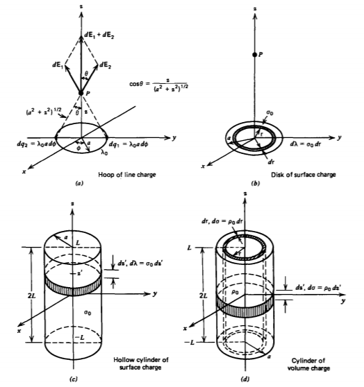
Figure 2-13b. Then the incremental z-directed electric field along the z axis due to a hoop of radius r is found from (14) as

\[dE_{z} = \frac{\sigma_{0} \textrm{r} z \: d \textrm{r}}{2 \varepsilon_{0} (\textrm{r}^{2} + z^{2})^{3/2}} \]

where we replace a with r, the radius of the incremental hoop. The total electric field is then

\[E_{z} = \frac{\sigma_{0}z}{2 \varepsilon_{0}} \int-{0}^{a} \frac{\textrm{r} d \textrm{r}}{(\textrm{r}^{2} + z^{2})^{3/2}} \\ = - \frac{\sigma_{0}z}{2 \varepsilon_{0}(\textrm{r}^{2} + z^{2})^{1/2}} \bigg|_{0}^{a} \\ = -\frac{\sigma_{0}}{2 \varepsilon_{0}} (\frac{z}{(a^{2} + z^{2})^{1/2}} - \frac{z}{\vert z \vert}) \\ = \pm \frac{\sigma_{0}}{2 \varepsilon_{0}} - \frac{\sigma_{0}z}{2 \varepsilon_{0}(a^{2} + z^{2})^{1/2}} \left \{ \begin{matrix} z > 0 \\ z< 0 \end{matrix} \right. \]

where care was taken at the lower limit (r = 0), as the magnitude of the square root must always be used.

As the radius of the disk gets very large, this result approaches that of the uniform field due to an infinite sheet of surface charge:

\[\lim_{a \rightarrow \infty} E_{z} = \pm \frac{\sigma_{0}}{2 \varepsilon_{0}} \left \{ \begin{matrix} z > 0 \\ z < 0 \end{matrix} \right. \]

(c) Hollow Cylinder of Surface Charge

A hollow cylinder of length 2L and radius a has its axis along the z direction and is centered about the z =0 plane as in Figure 2-13c. Its outer surface at r=a has a uniform distribution of surface charge \(\sigma_{0}\). It is necessary to distinguish between the coordinate of the field point z and the source point at z' (\(-L \leq z' \leq L\)). The hollow cylinder is broken up into incremental hoops of line charge \(d \lambda = \sigma_{0} dz'\). Then, the axial distance from the field point at z to any incremental hoop of line charge is (z -z'). The contribution to the axial electric field at z due to the incremental hoop at z' is found from (14) as'

\[dE_{z} = \frac{\sigma_{0}a(z-z') dz'}{2 \varepsilon_{0}[a^{2} + (z-z')^{2}]^{3/2}} \]

which when integrated over the length of the cylinder yields

\[E_{z} = \frac{\sigma_{0}a}{2 \varepsilon_{0}} \int_{-L}^{+L} \frac{(z-z') dz'}{[a^{2} + (z-z')^{2}]^{3/2}} \\ = \frac{\sigma_{0}a}{2 \varepsilon_{0}} \frac{1}{[a^{2} + (z - z')^{2}]^{1/2}} \bigg|_{z' = -L}^{+L} \\ = \frac{\sigma_{0}a}{2 \varepsilon_{0}} (\frac{1}{[a^{2} + (z-L)^{2}]^{1/2}} - \frac{1}{[a^{2} + (z + L)^{2}]^{1/2}}) \]

(d) Cylinder of Volume Charge

If this same cylinder is uniformly charged throughout the volume with charge density \(\rho_{0}\), we break the volume into differential-size hollow cylinders of thickness dr with incremental surface charge \(d \sigma = \rho_{0} d\) r as in Figure 2-13d. Then, the z-directed electric field along the z axis is obtained by integration of (21) replacing a by r:

\[E_{z} = \frac{\rho_{0}}{2 \varepsilon_{0}} \int_{0}^{a} \textrm{r}(\frac{1}{[\textrm{r}^{2} + (z - L)^{2}]^{1/2}} - \frac{1}{[\textrm{r}^{2} + (z + L)^{2}]^{1/2}}) d \textrm{r} \\ = \frac{\rho_{0}}{2 \varepsilon_{0}} \{[\textrm{r}^{2} + (z-L)^{2}]^{1/2} - [\textrm{r}^{2} + (z+L)^{2}]^{1/2} \} \bigg|_{0}^{a} \\ = \frac{\rho_{0}}{2 \varepsilon_{0}} \{[a^{2} + (z-L)^{2}]^{1/2} - \vert z - L \vert - [a^{2} + (z+L)^{2}]^{1/2} \\ + \vert z + L \vert \} \]

where at the lower r=0 limit we always take the positive square root.

This problem could have equally well been solved by breaking the volume charge distribution into many differential-sized surface charged disks at position z' (\(-L \leq z' \leq L\)), thickness dz', and effective surface charge density \(d \sigma = \rho_{0} dz'\). The field is then obtained by integrating (18).