2.2: The Coulomb Force Law Between Stationary Charges

Last updated
Save as PDF

Page ID: 48119

Markus Zahn
Massachusetts Institute of Technology via MIT OpenCourseWare

\( \newcommand{\vecs}[1]{\overset { \scriptstyle \rightharpoonup} {\mathbf{#1}} } \) \( \newcommand{\vecd}[1]{\overset{-\!-\!\rightharpoonup}{\vphantom{a}\smash {#1}}} \)\(\newcommand{\id}{\mathrm{id}}\) \( \newcommand{\Span}{\mathrm{span}}\) \( \newcommand{\kernel}{\mathrm{null}\,}\) \( \newcommand{\range}{\mathrm{range}\,}\) \( \newcommand{\RealPart}{\mathrm{Re}}\) \( \newcommand{\ImaginaryPart}{\mathrm{Im}}\) \( \newcommand{\Argument}{\mathrm{Arg}}\) \( \newcommand{\norm}[1]{\| #1 \|}\) \( \newcommand{\inner}[2]{\langle #1, #2 \rangle}\) \( \newcommand{\Span}{\mathrm{span}}\) \(\newcommand{\id}{\mathrm{id}}\) \( \newcommand{\Span}{\mathrm{span}}\) \( \newcommand{\kernel}{\mathrm{null}\,}\) \( \newcommand{\range}{\mathrm{range}\,}\) \( \newcommand{\RealPart}{\mathrm{Re}}\) \( \newcommand{\ImaginaryPart}{\mathrm{Im}}\) \( \newcommand{\Argument}{\mathrm{Arg}}\) \( \newcommand{\norm}[1]{\| #1 \|}\) \( \newcommand{\inner}[2]{\langle #1, #2 \rangle}\) \( \newcommand{\Span}{\mathrm{span}}\)\(\newcommand{\AA}{\unicode[.8,0]{x212B}}\)

Coulomb's Law

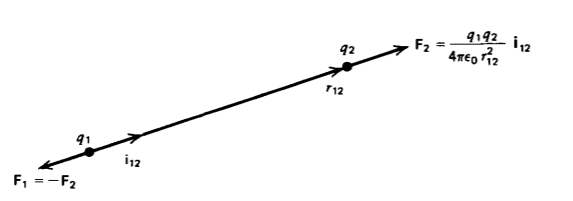
It remained for Charles Coulomb in 1785 to express these experimental observations in a quantitative form. He used a very sensitive torsional balance to measure the force between two stationary charged balls as a function of their distance apart. He discovered that the force between two small charges q₁ and q₂ (idealized as point charges of zero size) is proportional to their magnitudes and inversely proportional to the square of the distance r₁₂ between them, as illustrated in Figure 2-6. The force acts along the line joining the charges in the same or opposite direction of the unit vector i₁₂ and is attractive if the-charges are of opposite sign and repulsive if like charged. The force F₂ on charge q₂due to charge q_iis equal in magnitude but opposite in direction to the force F₁ on q₁, the net force on the pair of charges being zero.

\[\textbf{F}_{2} = - \textbf{F}_{1} = \frac{1}{4 \pi \varepsilon_{0}} \frac{q_{1}q_{2}}{r^{2}_{12}} \textbf{i}_{12} \textrm{nt} [\textrm{kg} - \textrm{m} - \textrm{s}^{-2}] \]

Units

The value of the proportionality constant \(1/4 \pi \varepsilon_{0}\) depends on the system of units used. Throughout this book we use SI units (Systeme International d'Unit6s) for which the base units are taken from the rationalized MKSA system of units where distances are measured in meters (m), mass in kilograms (kg), time in seconds (s), and electric current in amperes (A). The unit of charge is a coulomb where 1 coulomb= 1 ampere-second. The adjective "rationalized" is used because the factor of \(4 \pi\) is arbitrarily introduced into the proportionality factor in Coulomb's law of (1). It is done this way so as to cancel a \(4 \pi\) that will arise from other more often used laws we will introduce shortly. Other derived units are formed by combining base units.

Figure 2-6 The Coulomb force between two point charges is proportional to the magnitude of the charges and inversely proportional to the square of the distance between them. The force on each charge is equal in magnitude but opposite in direction. The force vectors are drawn as if q₁ and q₂ are of the same sign so that the charges repel. If q₁ and q₂ are of opposite sign, both force vectors would point in the opposite directions, as opposite charges attract.

The parameter \(\varepsilon_{0}\) is called the permittivity of free space and has a value

\[\varepsilon_{0} = (4 \pi \times 10^{-7} c^{2})^{-1} \\ \approx \frac{10^{-9}}{36 \pi} \approx 8.8542 \times 10^{-12} \textrm{farad}/\textrm{m} [\textrm{A}^{2} - \textrm{s}^{4} - \textrm{kg}^{-1} - \textrm{m}^{-3}] \]

where c is the speed of light in vacuum (\(c \approx 3 \times 10^{8}\) m/sec).

This relationship between the speed of light and a physical constant was an important result of the early electromagnetic theory in the late nineteenth century, and showed that light is an electromagnetic wave; see the discussion in Chapter 7.

To obtain a feel of how large the force in (1) is, we compare it with the gravitational force that is also an inverse square law with distance. The smallest unit of charge known is that of an electron with charge e and mass m_e

\(e \approx 1.60 \times 10^{-19} \: \textrm{Coul}, \: m_{e} \approx 9.11 \times 10^{-31} \textrm{kg}\)

Then, the ratio of electric to gravitational force magnitudes for two electrons is independent of their separation:

\[\frac{\textbf{F}_{e}}{\textbf{F}_{g}} = - \frac{e^{2}/(4 \pi \varepsilon_{0} r^{2})}{Gm_{e}^{2}/r^{2}} = - \frac{e^{2}}{m_{e}^{2}} \frac{1}{4 \pi \varepsilon_{0}G} \approx - 4.16 \times 10^{42} \]

where \(G = 6.67 \times 10^{-11} [\textrm{m}^{3} - \textrm{s}^{-2} - \textrm{kg}^{-1}]\) is the gravitational constant. This ratio is so huge that it exemplifies why electrical forces often dominate physical phenomena. The minus sign is used in (3) because the gravitational force between two masses is always attractive while for two like charges the electrical force is repulsive.

Electric Field

If the charge q₁ exists alone, it feels no force. If we now bring charge q₂ within the vicinity of q₁, then q₂ feels a force that varies in magnitude and direction as it is moved about in space and is thus a way of mapping out the vector force field due to q₁. A charge other than q₂ would feel a different force from q₂ proportional to its own magnitude and sign. It becomes convenient to work with the quantity of force per unit charge that is called the electric field, because this quantity is independent of the particular value of charge used in mapping the force field. Considering q₂ as the test charge, the electric field due to q₁ at the position of q₂ is defined as

\[\textrm{E}_{2} = \lim_{q_{2} \rightarrow 0} \frac{\textbf{F}_{2}}{q_{2}} = \frac{q_{1}}{4 \pi \varepsilon_{0} r^{2}_{12}} \textbf{i}_{12} \textrm{volts}/ \textrm{12} [\textrm{kg} - \textrm{m} - \textrm{s}^{-3} - \textrm{A}^{-1}] \]

In the definition of (4) the charge q₁ must remain stationary. This requires that the test charge q₂ be negligibly small so that its force on q₁ does not cause q₁ to move. In the presence of nearby materials, the test charge q₂ could also induce or cause redistribution of the charges in the material. To avoid these effects in our definition of the electric field, we make the test charge infinitely small so its effects on nearby materials and charges are also negligibly small. Then (4) will also be a valid definition of the electric field when we consider the effects of materials. To correctly map the electric field, the test charge must not alter the charge distribution from what it is in the absence of the test charge.

Superposition

If our system only consists of two charges, Coulomb's law (1) completely describes their interaction and the definition of an electric field is unnecessary. The electric field concept is only useful when there are large numbers of charge present as each charge exerts a force on all the others. Since the forces on a particular charge are linear, we can use superposition, whereby if a charge q₁ alone sets up an electric field E₁, and another charge q₂ alone gives rise to an electric field E₂, then the resultant electric field with both charges present is the vector sum E₁ +E₂. This means that if a test charge q_p is placed at point P in Figure 2-7, in the vicinity of N charges it will feel a force

\[\textbf{F}_{p} = q_{p} \textbf{E}_{P} \]

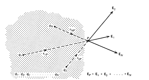
Figure 2-7 The electric field due to a collection of point charges is equal to the vector sum of electric fields from each charge alone.

where E_P is the vector sum of the electric fields due to all the N-point charges,

\[\textbf{E}_{P} = \frac{1}{4 \pi \varepsilon_{0}} (\frac{q_{1}}{r_{1P}^{2}} + \frac{q_{2}}{r_{2P}^{2}}\textbf{i}_{2P} + \frac{q_{3}}{r_{3P}^{2}} \textbf{i}_{3P} + ... +\frac{q_{N}}{r_{NP}^{2}} \textbf{i}_{NP}) = \frac{1}{4 \pi \varepsilon_{0}} \sum_{n = 1}^{N} \frac{q_{n}}{r^{2}_{nP}} \textbf{i}_{nP} \]

Note that E_P has no contribution due to q_psince a charge cannot exert a force upon itself.

Example 2-1: Two-Point Charges

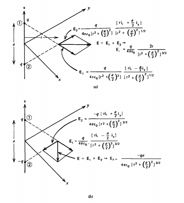
Two-point charges are a distance a apart along the z axis as shown in Figure 2-8. Find the electric field at any point in the z =0 plane when the charges are:

(a) both equal to q

(b) of opposite polarity but equal magnitude ±q. This configuration is called an electric dipole.

Solution

(a) In the z =0 plane, each point charge alone gives rise to field components in the i_r and i_z directions. When both charges are equal, the superposition of field components due to both charges cancel in the z direction but add radially:

\(E_{\textrm{r}}(z= 0) = \frac{q}{4 \pi \varepsilon_{0}} \frac{2 \textrm{r}}{[\textrm{r}^{2} + (a/2)^{2}]^{3/2}}\)

As a check note that far away from the point charges (r >> a) the field approaches that of a point charge of value 2q:

\(\lim_{r >>a} E_{\textrm{r}(z = 0) = \frac{2q}{4 \pi \varepsilon_{0}\textrm{r}^{2}}\)

(b) When the charges have opposite polarity, the total electric field due to both charges now cancel in the radial direction but add in the z direction:

\(E_{z}(z=0) = \frac{-q}{4 \pi \varepsilon_{0}} \frac{a}{[\textrm{r}^{2} + (a/2)^{2}]^{3/2}}\)

Far away from the point charges the electric field dies off as the inverse cube of distance:
\(\lim_{r >> a} E_{z} (z = 0) = \frac{-qa}{4 \pi \varepsilon_{0}\textrm{r}^{3}}\)

Figure 2-8 Two equal magnitude point charges are a distance a apart along the z axis. (a) When the charges are of the same polarity, the electric field due to each is radially directed away. In the z = 0 symmetry plane, the net field component is radial. (b) When the charges are of opposite polarity, the electric field due to the negative charge is directed radially inwards. In the z = 0 symmetry plane, the net field is now -z directed.

The faster rate of decay of a dipole field is because the net charge is zero so that the fields due to each charge tend to cancel each other out.