2.4: Gauss's Law

We could continue to build up solutions for given charge distributions using the coulomb superposition integral of Section 2.3.2. However, for geometries with spatial symmetry, there is often a simpler way using some vector properties of the inverse square law dependence of the electric field.

Properties of the Vector Distance Between Two Points, r_QP

(a) r_QP

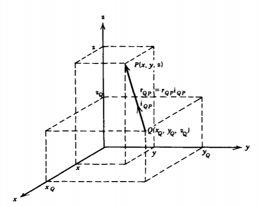
In Cartesian coordinates the vector distance r_QP between a source point at Q and a field point at P directed from Q to P as illustrated in Figure 2-14 is

\[\textbf{r}_{QP} = (x - x_{Q})\textbf{i}_{x} + (y - y_{q})\textbf{i}_{y} + (z-z_{Q})\textbf{i}_{z} \]

with magnitude

\[r_{QP} = [(x - x_{Q})^{2} + (y - y_{Q})^{2} + (z - z_{Q})^{2}]^{1/2} \]

The unit vector in the direction of \(\textbf{r}_{QP}\) is

\[\textbf{i}_{QP} = \frac{\textbf{r}_{QP}}{r_{QP}} \]

Figure 2-14 The vector distance r_QP between two points Q and P

(b) Gradient of the Reciprocal Distance, \(\nabla (1/r_{QP})\)

Taking the gradient of the reciprocal of (2) yields

\[\nabla(\frac{1}{r_{QP}}) = \textbf{i}_{x} \frac{\partial}{\partial x} (\frac{1}{r_{QP}}) + \textbf{i}_{y} \frac{\partial}{\partial y}(\frac{1}{r_{QP}}) + \textbf{i}_{z} \frac{\partial}{\partial z} (\frac{1}{r_{QP}}) \\ = -\frac{1}{r^{3}_{QP}} [(x - x_{Q})\textbf{i}_{x} + (y-y_{Q})\textbf{i}_{y} + (z - z_{Q}) \textbf{i}_{z}] \\ = - \textbf{i}_{QP}/r^{2}_{QP} \]

which is the negative of the spatially dependent term that we integrate to find the electric field in Section 2.3.2.

(c) Laplacian of the Reciprocal Distance

Another useful identity is obtained by taking the divergence of the gradient of the reciprocal distance. This operation is called the Laplacian of the reciprocal distance. Taking the divergence of (4) yields

\[\nabla^{2} (\frac{1}{r_{QP}}) = \nabla \cdot [\nabla (\frac{1}{r_{QP}})] \\ = \nabla \cdot (\frac{-\textbf{i}_{QP}}{r^{2}_{QP}}) \\ = -\frac{\partial}{\partial x} (\frac{x-x_{Q}}{r^{3}_{QP}}) - \frac{\partial}{\partial y} (\frac{y-y_{Q}}{r^{3}_{QP}}) - \frac{\partial}{\partial z} (\frac{z - z_{Q}}{r^{3}_{QP}}) \\ = - \frac{3}{r^{3}_{QP}} + \frac{3}{r^{5}_{QP}} [(x-x_{Q})^{2} + (y - y_{Q})^{2} + (z-z_{2})^{2}] \]

Using (2) we see that (5) reduces to

\[\nabla^{2} (\frac{1}{r_{QP}}) = \left \{ \begin{matrix} 0, & r_{QP} \neq 0 \\ \textrm{undefined} & r_{QP} = 0 \end{matrix} \right. \]

Thus, the Laplacian of the inverse distance is zero for all nonzero distances but is undefined when the field point is coincident with the source point.

Gauss's Law In Integral Form

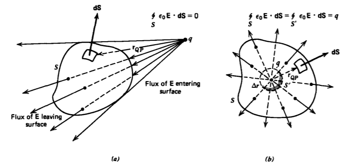
(a) Point Charge Inside or Outside a Closed Volume Now consider the two cases illustrated in Figure 2-15 where an arbitrarily shaped closed volume V either surrounds a point charge q or is near a point charge q outside the surface S. For either case the electric field emanates radially from the point charge with the spatial inverse square law. We wish to calculate the flux of electric field through the surface S surrounding the volume V:

\[\Phi = \oint_{S} \textbf{E} \cdot \textbf{dS} \\ = \oint_{S} \frac{q}{4 \pi \varepsilon_{0}r^{2}_{QP}} \textbf{i}_{QP} \cdot \textbf{dS} \\ = \oint_{S} \frac{-q}{4 \pi \varepsilon_{0}} \nabla (\frac{1}{r_{QP}}) \cdot \textbf{dS} \]

Figure 2-15 (a) The net flux of electric field through a closed surface S due to an outside point charge is zero because as much flux enters the near side of the surface as leaves on the far side. (b) All the flux of electric field emanating from an enclosed point charge passes through the surface.

where we used (4). We can now use the divergence theorem to convert the surface integral to a volume integral:

\[\oint_{S} \textbf{E} \cdot \textbf{dS} = \frac{-q}{4 \pi \varepsilon_{0}} \nabla \cdot [ \nabla (\frac{1}{r_{QP}})] dV \]

When the point charge q is outside the surface every point in the volume has a nonzero value of r_QP. Then, using (6) with \(r_{QP} \neq 0\), we see that the net flux of E through the surface is zero.

This result can be understood by examining Figure 2-15a. The electric field emanating from q on that part of the surface S nearest q has its normal component oppositely directed to dS giving a negative contribution to the flux. However, on the opposite side of S the electric field exits with its normal component in the same direction as dS giving a positive contribution to the flux. We have shown that these flux contributions are equal in magnitude but opposite in sign so that the net flux is zero.

As illustrated in Figure 2-15b, assuming q to be positive, we see that when S surrounds the charge the electric field points outwards with normal component in the direction of dS everywhere on S so that the flux must be positive. If q were negative, E and dS would be oppositely directed everywhere so that the flux is also negative. For either polarity with nonzero q, the flux cannot be zero. To evaluate the value of this flux we realize that (8) is zero everywhere except where r_QP =0 so that the surface S in (8) can be shrunk down to a small spherical surface S' of infinitesimal radius \(\Delta r\) surrounding the point charge; the rest of the volume has \(\r_{QP} \neq 0\) so that \(\nabla \cdot \nabla (1/r_{QP}) = 0\) On this incremental surface we know the electric field is purely radial in the same direction as dS' with the field due to a point charge:

\[\oint_{S} \textbf{E} \cdot \textbf{dS} = \oint_{S'} \textbf{E} \cdot \textbf{dS}' = \frac{q}{4 \pi \varepsilon_{0}(\Delta r)^{2}} 4 \pi (\Delta r)^{2} = \frac{q}{\varepsilon_{0}} \]

If we had many point charges within the surface S, each charge q_i gives rise to a flux \(q_{i}/ \varepsilon_{0}\) so that Gauss's law states that the net flux of \(\varepsilon_{0}\textbf{E}\) through a closed surface is equal to the net charge enclosed by the surface:

\[\oint_{S} \varepsilon_{0} \textbf{E} \cdot \textbf{dS} = \sum_{\textrm{all } q_{i} \textrm{ inside } S} q_{i} \]

Any charges outside S do not contribute to the flux

(b) Charge Distributions

For continuous charge distributions, the right-hand side of (10) includes the sum of all enclosed incremental charge elements so that the total charge enclosed may be a line, surface, and/or volume integral in addition to the sum of point charges:

\[\oint_{S} \varepsilon_{0} \textbf{E} \cdot \textbf{dS} = \sum_{\textrm{all } q_{i} \textrm{ inside } S} q_{i} + \int_{\textrm{all } q \textrm{ inside} S} dq \\ = (\sum q_{i} + \int_{L} \lambda dl + \int_{S} \sigma d \textrm{S} + \int_{\textrm{V}} \rho d \textrm{V} \bigg|_{\textrm{all charge inside} S} \]

Charges outside the volume give no contribution to the total flux through the enclosing surface.

Gauss's law of (11) can be used to great advantage in simplifying computations for those charges distributed with spatial symmetry. The trick is to find a surface S that has sections tangent to the electric field so that the dot product is zero, or has surfaces perpendicular to the electric field and upon which the field is constant so that the dot product and integration become pure multiplications. If the appropriate surface is found, the surface integral becomes very simple to evaluate.

Coulomb's superposition integral derived in Section 2.3.2 is often used with symmetric charge distributions to determine if any field components are zero. Knowing the direction of the electric field often suggests the appropriate Gaussian surface upon which to integrate (11). This integration is usually much simpler than using Coulomb's law for each charge element

Spherical Symmetry

(a) Surface Charge

A sphere of radius R has a uniform distribution of surface charge \(\sigma_{0}\) as in Figure 2-16a. Measure the angle \(\theta\) from the line joining any point P at radial distance r to the sphere center. Then, the distance from P to any surface charge element on the sphere is independent of the angle \(\phi\). Each differential surface charge element at angle \(\theta\) contributes field components in the radial and \(\theta\) directions, but symmetrically located charge elements at -\(\phi\) have equal field magnitude components that add radially but cancel in the \(\theta\) direction.

Realizing from the symmetry that the electric field is purely radial and only depends on r and not on \(\theta\) or \(\phi\), we draw Gaussian spheres of radius r as in Figure 2-16b both inside (r < R) and outside (r>R) the charged sphere. The Gaussian sphere inside encloses no charge while the outside sphere

Figure 2-16 A sphere of radius R with uniformly distributed surface charge \(\sigma_{0}\). (a) Symmetrically located charge elements show that the electric field is purely radial. (b) Gauss's law, applied to concentric spherical surfaces inside (r < R) and outside (r > R) the charged sphere, easily shows that the electric field within the sphere is zero and outside is the same as if all the charge \(Q = 4 \pi R^{2} \sigma_{0}\) were concentrated as a point charge at the origin.

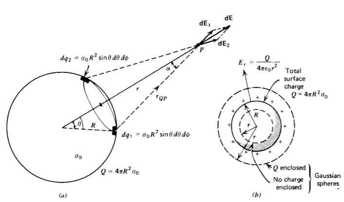
encloses all the charge \(Q = \sigma_{0} 4 \pi R^{2}\):

\[\oint_{S} \varepsilon_{0} \textbf{E} \cdot \textbf{dS} = \varepsilon_{0} E_{r} 4 \pi r^{2} = \left \{ \begin{matrix} \sigma_{0} 4 \pi R^{2} = Q, & r > R \\ 0, & r<R \end{matrix} \right. \]

so that the electric field is

\[E_{r} = \left \{ \begin{matrix} \frac{\sigma_{0}R^{2}}{\varepsilon_{0}r^{2}} = \frac{Q}{4 \pi \varepsilon_{0}r^{2}}, & r > R \\ 0, & r<R \end{matrix} \right. \]

The integration in (12) amounts to just a multiplication of \(\varepsilon_{0}E_{r}\), and the surface area of the Gaussian sphere because on the sphere the electric field is constant and in the same direction as the normal ir. The electric field outside the sphere is the same as if all the surface charge were concentrated as a point charge at the origin.

The zero field solution for r < R is what really proved Coulomb's law. After all, Coulomb's small spheres were not really point charges and his measurements did have small sources of errors. Perhaps the electric force only varied inversely with distance by some power close to two, \(r^{-2 + \delta}\), where \(\delta\) is very small. However, only the inverse square law gives a zero electric field within a uniformly surface charged sphere. This zero field result is true for any closed conducting body of arbitrary shape charged on its surface with no enclosed charge. Extremely precise measurements were made inside such conducting surface charged bodies and the electric field was always found to be zero. Such a closed conducting body is used for shielding so that a zero field environment can be isolated and is often called a Faraday cage, after Faraday's measurements of actually climbing into a closed hollow conducting body charged on its surface to verify the zero field results.

To appreciate the ease of solution using Gauss's law, let us redo the problem using the superposition integral of Section 2.3.2. From Figure 2-16a the incremental radial component of electric field due to a differential charge element is

\[dE_{r} = \frac{\sigma_{0}R^{2} \sin \theta \: d \theta \: d \phi}{4 \pi \varepsilon_{0}r^{2}_{QP}} \cos \alpha \]

From the law of cosines the angles and distances are related as

\[r_{QP}^{2} = r^{2} + R^{2} - 2rR \: \cos \: \theta \\ R^{2} = r^{2} + r_{QP}^{2} - 2 r r_{QP} \cos \: \alpha \]

so that \(\alpha\) is related to \(\theta\) as

\[\cos \alpha = \frac{r - R \cos \theta}{[r^{2} + R^{2} - 2 r R \: \cos \theta]^{1/2}} \]

Then the superposition integral of Section 2.3.2 requires us to integrate (14) as

\[E_{r} = \int_{\theta = 0}^{\pi} \int_{\phi = 0}^{2 \pi} \frac{\sigma_{0}R^{2} \sin \: \theta (r-R \: \cos \: \theta) d \theta d \phi}{4 \pi \varepsilon_{0}[r^{2} + R^{2} - 2rR \: \cos \: \theta]^{3/2}} \]

After performing the easy integration over \(\phi\) that yields the factor of \(2 \pi\), we introduce the change of variable:

\[u = r^{2} + R^{2} - 2 r R \: \cos \: \theta \\ du = 2 r R \: \sin \theta \: d \theta \]

which allows us to rewrite the electric field integral as

\[E_{r} = \int_{u = (r-R)^{2}}^{(r + R)^{2}} \frac{\sigma_{0}R[u + r^{2} - R^{2}] du}{8 \varepsilon_{0}r^{2}u^{3/2}} \\ = \frac{\sigma_{0}R}{4 \varepsilon_{0} r^{2}} (u^{1/2} - \frac{(r^{2}-R^{2})}{u^{1/2}} ) \bigg|_{(r-R)^{2}}^{(r + R)^{2}} \\ = \frac{\sigma_{0}R}{4 \varepsilon_{0}r^{2}}[(r + R) - \vert r - R \vert - (r^{2} - R^{2}) (\frac{1}{r + R} - \frac{1}{\vert r - R \vert})] \]

where we must be very careful to take the positive square root in evaluating the lower limit of the integral for r < R. Evaluating (19) for r greater and less than R gives us (13), but with a lot more effort.

(b) Volume Charge Distribution

If the sphere is uniformly charged throughout with density \(\rho_{0}\), then the Gaussian surface in Figure 2-17a for r > R still encloses the total charge \(Q = \frac{4}{3} \pi R^{3} \rho_{0}\). However, now the smaller Gaussian surface with r < R encloses a fraction of the total charge:

\[\oint_{S} \varepsilon_{0} \textbf{E} \cdot \textbf{dS} = \varepsilon_{0}E_{r} 4 \pi r^{2} = \left \{ \begin{matrix} \rho_{0} \frac{4}{3} \pi r^{3} = Q(r/R)^{3}, & r<R \\ \rho_{0}\frac{4}{3} \pi R^{3} = Q, & r>R \end{matrix} \right. \]

Figure 2-17 (a) Gaussian spheres for a uniformly charged sphere show that the electric field outside the sphere is again the same as if all the charge \(Q = \frac{4}{3} \pi R^{3} \rho_{0}\) were concentrated as a point charge at r =0. (b) The solution is also obtained by summing the contributions from incremental spherical shells of surface charge.

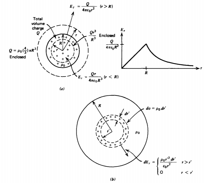
so that the electric field is

\[E_{r} = \left \{ \begin{matrix} \frac{\rho_{0}r}{3 \varepsilon_{0}} = \frac{Qr}{4 \pi \varepsilon_{0} R^{3}}, & r < R \\ \frac{\rho_{0}R^{3}}{3 \varepsilon_{0}r^{2}} = \frac{Q}{4 \pi \varepsilon_{0}r^{2}}, & r > R \end{matrix} \right. \]

This result could also have been obtained using the results of (13) by breaking the spherical volume into incremental shells of radius r', thickness dr', carrying differential surface charge \(d \sigma = \rho_{0} dr'\) as in Figure 2-17b. Then the contribution to the field is zero inside each shell but nonzero outside:

\[dE_{r} = \left \{ \begin{matrix} 0, & r<r' \\ \frac{\rho_{0}r'^{2} dr'}{\varepsilon_{0}r^{2}}, & r>r' \end{matrix} \right. \]

The total field outside the sphere is due to all the differential shells, while the field inside is due only to the enclosed shells:

\[E_{r} = \left \{ \begin{matrix} \int_{0}^{r} \frac{r'^{2}\rho_{0}dr'}{\varepsilon_{0}r^{2}} = \frac{\rho_{0}r}{3 \varepsilon_{0}} = \frac{Qr}{4 \pi \varepsilon_{0}R^{3}}, & r<R \\ \int_{0}^{R} \frac{r'^{2} \rho_{0}dr'}{\varepsilon_{0}r^{2}} = \frac{\rho_{0}R^{3}}{3 \varepsilon_{0}r^{2}} = \frac{Q}{4 \pi \varepsilon_{0}r^{2}}, & r>R \end{matrix} \right. \]

which agrees with (21)

Cylindrical Symmetry

(a) Hollow Cylinder of Surface Charge

An infinitely long cylinder of radius a has a uniform distribution of surface charge \(\sigma_{0}\), as shown in Figure 2-18a. The angle \(\phi\) is measured from the line joining the field point P to the center of the cylinder. Each incremental line charge element \(d \lambda = \sigma_{0}a \: d \phi\) do contributes to the electric field at P as given by the solution for an infinitely long line charge in Section 2.3.3. However, the symmetrically located element at \(-\phi\) gives rise to equal magnitude field components that add radially as measured from the cylinder center but cancel in the \(\phi\) direction

Because of the symmetry, the electric field is purely radial so that we use Gauss's law with a concentric cylinder of radius r and height L, as in Figure 2-18b where L is arbitrary. There is no contribution to Gauss's law from the upper and lower surfaces because the electric field is purely tangential. Along the cylindrical wall at radius r, the electric field is constant and

Figure 2-18 (a) Symmetrically located line charge elements on a cylinder with uniformly distributed surface charge show that the electric field is purely radial. (b) Gauss's law applied to concentric cylindrical surfaces shows that the field inside the surface charged cylinder is zero while outside it is the same as if all the charge per unit length \(\sigma_{0} 2 \pi a\) were concentrated at the origin as a line charge. (c) In addition to using the surfaces of (b) with Gauss's law for a cylinder of volume charge, we can also sum the contributions from incremental hollow cylinders of surface charge.

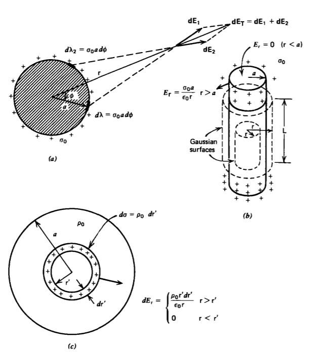
purely normal so that Gauss's law simply yields

\[\oint_{S} \varepsilon_{0} \textbf{E} \cdot \textbf{dS} = \varepsilon_{0} L_{\textrm{r}} 2 \pi \textrm{r} L = \left \{ \begin{matrix} \sigma_{0} 2 \pi aL, & \textrm{r} > a \\ 0 & \textrm{r} < a \end{matrix} \right. \]

where for r<a all the charge within a height L is enclosed. The electric field outside the cylinder is then the same as if all the charge per unit length \(\lambda = \sigma_{0} 2 \pi a\) were concentrated along the axis of the cylinder:

\[E_{r} = \left \{ \begin{matrix} \frac{\sigma_{0}a}{\varepsilon_{0} \textrm{r}} = \frac{\lambda}{2 \pi \varepsilon_{0} \textrm{r}} & \textrm{r} > a \\ 0, & \textrm{r} < a \end{matrix} \right. \]

Note in (24) that the arbitrary height L canceled out.

(b) Cylinder of Volume Charge

If the cylinder is uniformly charged with density \(\rho_{0}\), both Gaussian surfaces in Figure 2-18b enclose charge

\oint_S \varepsilon_0 \mathbf{E} \cdot \mathbf{d S}=\varepsilon_0 E_{\mathrm{r}} 2 \pi \mathrm{r} L=\left\{\begin{array}{ll}
\rho_0 \pi a^2 L, & \mathrm{r}>a \\
\rho_0 \pi \mathrm{r}^2 L, & \mathrm{r}<a
\end{array}\right.

so that the electric field is

\[E_{\textrm{r}} = \left \{ \begin{matrix} \frac{\rho_{0}a^{2}}{2 \varepsilon_{0} \textrm{r}} = \frac{\lambda}{2 \pi \varepsilon_{0} \textrm{r}}, & \textrm{r} > a \\ \frac{\rho_{0} \textrm{r}}{2 \varepsilon_{0}} = \frac{\lambda \textrm{r}}{2 \pi \varepsilon_{0} a^{2}} & \textrm{r} < a \end{matrix} \right. \]

where \(\lambda = \rho_{0} \pi a^{2}\) is the total charge per unit length on the cylinder.

Of course, this result could also have been obtained by integrating (25) for all differential cylindrical shells of radius r' with thickness d r' carrying incremental surface charge \(d \sigma = \rho_{0} d \textrm{r}'\), as in Figure 2-18c

\[E_{\textrm{r}} = \left \{ \begin{matrix} \int_{0}^{a} \frac{\rho_{0}\textrm{r}'}{\varepsilon_{0}\textrm{r}} d \textrm{r}' = \frac{\rho_{0}}{2 \varepsilon_{0} \textrm{r}} = \frac{\lambda}{2 \pi \varepsilon_{0} \textrm{r}}, & \textrm{r} > a \\ \int_{0}^{\textrm{r}} \frac{\rho_{0} \textrm{r}'}{\varepsilon_{0} \textrm{r}} d \textrm{r}' = \frac{\rho_{0} \textrm{r}}{2 \varepsilon_{0}} = \frac{\lambda \textrm{r}}{2 \pi \varepsilon_{0} a^{2}}, & \textrm{r} < a \end{matrix} \right. \]

Gauss's Law and the Divergence Theorem

If a volume distribution of charge \(\rho\) is completely surrounded by a closed Gaussian surface S, Gauss's law of (11) is

\[ \oint_S \varepsilon_0 \mathbf{E} \cdot \mathbf{d S}=\int_V \rho d V \]

The left-hand side of (29) can be changed to a volume integral using the divergence theorem:

\[\oint_{S} \varepsilon_{0} \textbf{E} \cdot \textbf{dS} = \int_{V} \nabla \cdot (\varepsilon_{0} \textbf{E}) dV = \int_{V} \rho d V \]

Since (30) must hold for any volume, the volume integrands in (30) must be equal, yielding the point form of Gauss's law:

\[ \nabla \cdot\left(\varepsilon_0 \mathbf{E}\right)=\rho \]

Since the permitivity of free space \(\varepsilon_{0}\) is a constant, it can freely move outside the divergence operator.

Electric Field Discontinuity Across a Sheet of Surface Charge

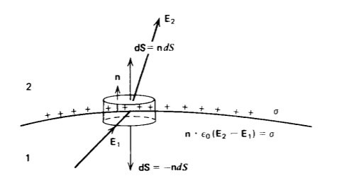
In Section 2.3.4a we found that the electric field changes direction discontinuously on either side of a straight sheet of surface charge. We can be more general by applying the surface integral form of Gauss's law in (30) to the differential-sized pill-box surface shown in Figure 2-19 surrounding a small area dS of surface charge

\[\oint_{S} \varepsilon_{0} \textbf{E} \cdot \textbf{dS} = \int_{S} \sigma d S \Rightarrow \varepsilon_{0} (E_{2n} - E_{1n}) dS = \sigma dS \]

where E_2n and E_1n are the perpendicular components of electric field on each side of the interface. Only the upper and lower surfaces of the pill-box contribute in (32) because the surface charge is assumed to have zero thickness so that the short cylindrical surface has zero area. We thus see that the surface charge density is proportional to the discontinuity in the normal component of electric field across the sheet:

\[\varepsilon_{0}(E_{2n} - E_{1n}) = \sigma \Rightarrow \textbf{n} \cdot \varepsilon_{0}(\textbf{E}_{2} - \textbf{E}_{1}) = \sigma \]

where n is perpendicular to the interface directed from region 1 to region 2.

Figure 2-19 Gauss's law applied to a differential sized pill-box surface enclosing some surface charge shows that the normal component of \(\varepsilon_{0}\textbf{E}\) is discontinuous in the surface charge density.