2.5: The Electric Potential

If we have two charges of opposite sign, work must be done to separate them in opposition to the attractive coulomb force. This work can be regained if the charges are allowed to come together. Similarly, if the charges have the same sign, work must be done to push them together; this work can be regained if the charges are allowed to separate. A charge gains energy when moved in a direction opposite to a force. This is called potential energy because the amount of energy depends on the position of the charge in a force field.

Work Required to Move a Point Charge

The work W required to move a test charge q_t along any path from the radial distance r_a to the distance r_b with a force that just overcomes the coulombic force from a point charge q, as shown in Figure 2-20, is

\[W = - \int_{r_{a}}^{r_{b}} \textbf{F} \cdot \textbf{dl} \\ = -\frac{qq_{t}}{4 \pi \varepsilon_{0}} \int_{r_{a}}^{r_{b}} \frac{\textbf{i}_{r} \cdot \textbf{dl}}{r^{2}} \]

Figure 2-20 It takes no work to move a test charge q_t along the spherical surfaces perpendicular to the electric field due to a point charge q. Such surfaces are called equipotential surfaces.

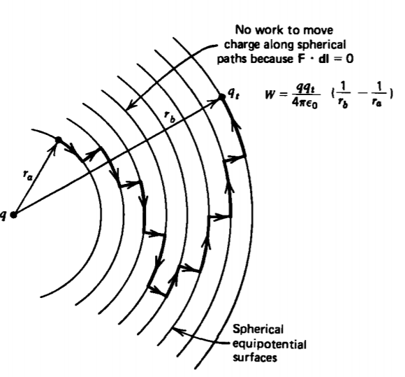
The minus sign in front of the integral is necessary because the quantity W represents the work we must exert on the test charge in opposition to the coulombic force between charges. The dot product in (1) tells us that it takes no work to move the test charge perpendicular to the electric field, which in this case is along spheres of constant radius. Such surfaces are called equipotential surfaces. Nonzero work is necessary to move q to a different radius for which \(\textbf{dl} = dr \textbf{i}_{r}\). Then, the work of (1) depends only on the starting and ending positions (r_a and r_b) of the path and not on the shape of the path itself:

\[W = - \frac{qq_{t}}{4 \pi \varepsilon_{0}} \int_{r_{a}}^{r_{b}} \frac{dr}{r^{2}} \\ = \frac{qq_{t}}{4 \pi \varepsilon_{0}} (\frac{1}{r_{b}} - \frac{1}{r_{a}}) \]

We can convince ourselves that the sign is correct by examining the case when r_b is bigger than r_a and the charges q and q_t are of opposite sign and so attract each other. To separate the charges further requires us to do work on q_t so that W is positive in (2). If q and q_t are the same sign, the repulsive coulomb force would tend to separate the charges further and perform work on q_t. For force equilibrium, we would have to exert a force opposite to the direction of motion so that W is negative.

If the path is closed so that we begin and end at the same point with r_a = r_b, the net work required for the motion is zero. If the charges are of the opposite sign, it requires positive work to separate them, but on the return, equal but opposite work is performed on us as the charges attract each other.

If there was a distribution of charges with net field E, the work in moving the test charge against the total field E is just the sum of the works necessary to move the test charge against the field from each charge alone. Over a closed path this work remains zero:

\[W= \oint_{L} - q_{t} \textbf{E} \cdot \textbf{dl} = 0 \Rightarrow \oint_{L} \textbf{e} \cdot \textbf{dl} = 0 \]

which requires that the line integral of the electric field around the closed path also be zero.

Electric Field and Stokes' Theorem

Using Stokes' theorem of Section 1.5.3, we can convert the line integral of the electric field to a surface integral of the curl of the electric field:

\[\oint_{L} \textbf{E} \cdot \textbf{dl} = \int_{S} (\nabla \times \textbf{E}) \cdot \textbf{dS} \]

From Section 1.3.3, we remember that the gradient of a scalar function also has the property that its line integral around a closed path is zero. This means that the electric field can be determined from the gradient of a scalar function V called the potential having units of volts [kg-m²-s^-3-A^-1]:

\[\textbf{E} = - \nabla V \]

The minus sign is introduced by convention so that the electric field points in the direction of decreasing potential. From the properties of the gradient discussed in Section 1.3.1 we see that the electric field is always perpendicular to surfaces of constant potential.

By applying the right-hand side of (4) to an area of differential size or by simply taking the curl of (5) and using the vector identity of Section 1.5.4a that the curl of the gradient is zero, we reach the conclusion that the electric field has zero curl:

\[\nabla \times \textbf{E} = 0 \]

Potential and the Electric Field

The potential difference between the two points at r_a and r_b is the work per unit charge necessary to move from r_a to r_b:

\[V(r_{b}) - V(r_{a}) = \frac{W}{q_{t}} \\ = - \int_{r_{a}}^{r_{b}} \textbf{E} \cdot \textbf{dl} = + \int_{r_{b}}^{r_{a}} \textbf{E} \cdot \textbf{dl} \]

Note that (3), (6), and (7) are the fields version of Kirchoff's circuit voltage law that the algebraic sum of voltage drops around a closed loop is zero.

The advantage to introducing the potential is that it is a scalar from which the electric field can be easily calculated. The electric field must be specified by its three components, while if the single potential function V is known, taking its negative gradient immediately yields the three field components. This is often a simpler task than solving for each field component separately. Note in (5) that adding a constant to the potential does not change the electric field, so the potential is only uniquely defined to within a constant. It is necessary to specify a reference zero potential that is often taken at infinity. In actual practice zero potential is often assigned to the earth's surface so that common usage calls the reference point "ground."

The potential due to a single point charge q is

\[V(r_{b}) - V(r_{a}) = - \int_{r_{a}}^{r_{b}} \frac{q \: dr}{4 \pi \varepsilon_{0}r^{2}} = \frac{q}{4 \pi \varepsilon_{0}r} \bigg|_{r_{a}}^{r_{b}} \\ = \frac{q}{4 \pi \varepsilon_{0}} (\frac{1}{r_{b}} - \frac{1}{r_{a}}) \]

If we pick our reference zero potential at \(r_{a} = \infty\), \(V(r_{a}) = 0\) so that \(r_{b} = r\) is just the radial distance from the point charge. The scalar potential V is then interpreted as the work per unit charge necessary to bring a charge from infinity to some distance r from the point charge q:

\[V(r) = \frac{q}{4 \pi \varepsilon_{0}r} \]

The net potential from many point charges is obtained by the sum of the potentials from each charge alone. If there is a continuous distribution of charge, the summation becomes an integration over all the differential charge elements dq:

\[V = \int_{\textrm{all} q} \frac{dq}{4 \pi \varepsilon_{0} r_{QP}} \]

where the integration is a line integral for line charges, a surface integral for surface charges, and a volume integral for volume charges.

The electric field formula of Section 2.3.2 obtained by superposition of coulomb's law is easily re-obtained by taking the negative gradient of (10), recognizing that derivatives are to be taken with respect to field positions (x, y, z) while the integration is over source positions (x_Q, y_Q, z_Q). The del operator can thus be brought inside the integral and operates only on the quantity r_QP:

\[\textbf{E} = -\nabla V = - \int_{\textbf{all } q} \frac{dq}{4 \pi \varepsilon_{0}} \nabla (\frac{1}{r_{QP}}) \\ = \int_{\textrm{all } q} \frac{dq}{4 \pi \varepsilon_{0} r^{2}_{QP}} \textbf{i}_{QP} \]

where we use the results of Section 2.4.1b for the gradient of the reciprocal distance.

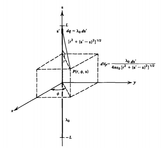
Finite Length Line Charge

To demonstrate the usefulness of the potential function, consider the uniform distribution of line charge \(\lambda_{0}\) of finite length 2L centered on the z axis in Figure 2-21. Distinguishing between the position of the charge element \(dq = \lambda_{0} dz'\) at z' and the field point at coordinate z, the distance between source and field point is

\[r_{QP} = [\textrm{r}^{2} + (z - z')^{2}]^{1/2} \]

Substituting into (10) yields

\[V = \int_{-L}^{L} \frac{\lambda_{0}dz'}{4 \pi \varepsilon_{0}[\textrm{r}^{2} + (z-z')^{2}]^{1/2}} \\ = - \frac{\lambda_{0}}{4 \pi \varepsilon_{0}} \ln (\frac{z - L + [\textrm{r}^{2} + (z-L)^{2}]^{1/2}}{z + L + [\textrm{r}^{2} + (z+L)^{2}]^{1/2}}) \\ = - \frac{\lambda_{0}}{4 \pi \varepsilon_{0}}(\sinh^{-1} \frac{z -L}{\textrm{r}} - \sinh^{-1} \frac{z + L}{\textrm{r}}) \]

Figure 2-21 The potential from a finite length of line charge is obtained by adding the potentials due to each incremental line charge element.

The field components are obtained from (13) by taking the negative gradient of the potential:

\[E_{z} = -\frac{\partial V}{\partial z} = \frac{\lambda_{0}}{4 \pi \varepsilon_{0}} (\frac{1}{[\textrm{r}^{2} + (z-L)^{2}]^{1/2}} - \frac{1}{[\textrm{r}^{2} + (z + L)^{2}]^{1/2}}) \\ E_{\textrm{r}} = -\frac{\partial V}{\partial \textrm{r}} = \frac{\lambda_{0} \textrm{r}}{4 \pi \varepsilon_{0}} (\frac{1}{[\textrm{r}^{2} + (z-L)^{2}]^{1/2}[z-L + [\textrm{r}^{2} + (z-L)^{2}]^{1/2}]} \\ - \frac{1}{[\textrm{r}^{2} + (z+L)^{2}]^{1/2} [z+L + [\textrm{r}^{2} + (z+L)^{2}]^{1/2}]}) \\ = - \frac{\lambda_{0}}{4 \pi \varepsilon_{0}\textrm{r}} (\frac{z-L}{[\textrm{r}^{2} + (z-L)^{2}]^{1/2}} - \frac{z+L}{[\textrm{r}^{2} + (z+L)^{2}]^{1/2}}) \]

As L becomes large, the field and potential approaches that of an infinitely long line charge:

\[\lim_{L \rightarrow \infty} \left \{ \begin{matrix} E_{z} = 0 \\ E_{\textrm{r}} = \frac{\lambda_{0}}{2 \pi \varepsilon_{0}\textrm{r}} \\ V = - \frac{\lambda_{0}}{2 \pi \varepsilon_{0}} (\ln \textrm{r} - \ln 2L) \end{matrix} \right. \]

The potential has a constant term that becomes infinite when L is infinite. This is because the zero potential reference of (10) is at infinity, but when the line charge is infinitely long the charge at infinity is nonzero. However, this infinite constant is of no concern because it offers no contribution to the electric field.

Far from the line charge the potential of (13) approaches that of a point charge \(2 \lambda_{0}L\):

\[\lim_{r^{2} = \textrm{r}^{2} = z^{2} >> L^{2}} V = \frac{\lambda_{0}(2L)}{4 \pi \varepsilon_{0}r} \]

Other interesting limits of (14) are

\[\lim_{z = 0} \left \{ \begin{array}{ll} E_{z} = 0 \\ E_{\textrm{r}} = \frac{\lambda_{0}L}{2 \pi \varepsilon_{0}\textrm{r}(\textrm{r}^{2} + L^{2})^{1/2}} \end{array} \right. \\ \\ \lim_{\textrm{r} = 0} \left \{ \begin{array}{ll} E_{z} = \frac{\lambda_{0}}{4 \pi \varepsilon_{0}} (\frac{1}{\vert z - L \vert} - \frac{1}{\vert z + L \vert}) = \left \{ \begin{array}{ll} \frac{\pm \lambda_{0}L}{2 \pi \varepsilon_{0}(z^{2} - L^{2})}, & \left. \begin{array}{ll} z> L \\ z< -L \end{array} \right. \\ \frac{\lambda_{0}z}{2 \pi \varepsilon_{0}(L^{2}-z^{2})}, & -L \leq z \leq L \end{array} \right. \\ E_{\textrm{r}} = 0 \end{array} \right. \]

Charged Spheres

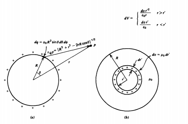
(a) Surface Charge A sphere of radius R supports a uniform distribution of surface charge ao with total charge \(Q = \sigma_{0} 4 \pi R^{2}\), as shown in Figure 2-22a. Each incremental surface charge element contributes to the potential as

\[dV = \frac{\sigma_{0}R^{2} \sin \theta \: d \theta \: d \phi}{4 \pi \varepsilon_{0} r_{QP}} \]

where from the law of cosines

\[r_{QP}^{2} =R^{2} + r^{2} - 2 r R \cos \theta \]

so that the differential change in \(r_{QP}\) about the sphere is

\[2r_{QP}dr_{QP} = 2rR \sin \: \theta \: d \theta \]

Figure 2-22 (a) A sphere of radius R supports a uniform distribution of surface charge \(\sigma_{0}\). (b) The potential due to a uniformly volume charged sphere is found by summing the potentials due to differential sized shells.

Therefore, the total potential due to the whole charged sphere is

\[V = \int_{r_{QP} = \vert r - R \vert}^{r + R} \int_{\phi = 0}^{2 \pi} \frac{\sigma_{0}R}{4 \pi \varepsilon_{0}r} dr_{QP} d\phi \\ = \frac{\sigma_{0}R}{2 \varepsilon_{0}r} r_{QP} \bigg|_{\vert r - R \vert}^{r + R} \\ = \left \{ \begin{matrix} \frac{\sigma_{0}R^{2}}{\varepsilon_{0}r} = \frac{q}{4 \pi \varepsilon_{0}r}, & r > R \\ \frac{\sigma_{0}R}{\varepsilon_{0}} = \frac{Q}{4 \pi \varepsilon_{0}R}, & r<R \end{matrix} \right. \]

Then, as found in Section 2.4.3a the electric field is
\[
E_{\mathrm{r}}=-\frac{\partial V}{\partial r}=\left\{\begin{array}{ll}
\frac{\sigma_0 R^2}{\varepsilon_0 r^2}=\frac{Q}{4 \pi \varepsilon_0 r^2}, & r>R \\
0 & r<R
\end{array}\right.
\]

Outside the sphere, the potential of (21) is the same as if all the charge Q were concentrated at the origin as a point charge, while inside the sphere the potential is constant and equal to the surface potential.

(b) Volume Charge

If the sphere is uniformly charged with density \(\rho_{0}\) and total charge \(Q = \frac{4}{3} \pi R^{3} \rho_{0}\), the potential can be found by breaking the sphere into differential size shells of thickness dr' and incremental surface charge \(d \sigma = \rho_{0} \: dr'\). Then, integrating (21) yields

\[V = \left \{ \begin{matrix} \int_{0}^{R} \frac{\rho_{0}r'^{2}}{\varepsilon_{0}r} dr' = \frac{\rho_{0}R^{3}}{3 \varepsilon_{0}r} = \frac{Q}{4 \pi \varepsilon_{0}r}, & r>R \\ \int_{0}^{r} \frac{\rho_{0}r'^{2}}{\varepsilon_{0}r} dr' + \int_{r}^{R} \frac{\rho_{0}r'}{\varepsilon_{0}} dr' = \frac{\rho_{0}}{2 \varepsilon_{0}}(R^{2} - \frac{r^{2}}{3}) \end{matrix} \right. \\ = \frac{3Q}{8 \pi \varepsilon_{0} R^{3}}(R^{2} - \frac{r^{2}}{3}) \: \: \: r <R \]

where we realized from (21) that for r < R the interior shells have a different potential contribution than exterior shells.

Then, the electric field again agrees with Section 2.4.3b:

\[E_{r} = - \frac{\partial V}{\partial r} = \left \{ \begin{matrix} \frac{\rho_{0}R^{3}}{3 \varepsilon_{0}r^{2}} = \frac{Q}{4 \pi \varepsilon_{0}r^{2}}, & r>R \\ \frac{\rho_{0}r}{3 \varepsilon_{0}} = \frac{Qr}{4 \pi \varepsilon_{0}R^{3}}, & r<R \end{matrix} \right. \]

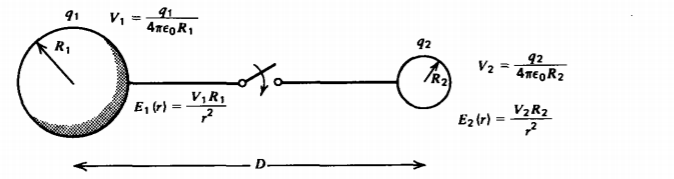
(c) Two Spheres

Two conducting spheres with respective radii R₁ and R₂ have their centers a long distance D apart as shown in Figure 2-23. Different charges Q₁ and Q₂ are put on each sphere. Because \(D >> R_{1} = R_{2}\), each sphere can be treated as isolated. The potential on each sphere is then

\[V_{1} = \frac{Q_{1}}{4 \pi \varepsilon_{0}R_{1}}, \: \: \: \: V_{2} = \frac{Q_{2}}{4 \pi \varepsilon_{0}R_{2}} \]

If a wire is connected between the spheres, they are forced to be at the same potential:

\[V_{0} = \frac{q_{1}}{4 \pi \varepsilon_{0}R_{1}} = \frac{q_{2}}{4 \pi \varepsilon_{0}R_{2}} \]

causing a redistribution of charge. Since the total charge in the system must be conserved,

\[q_{1} + q_{2} = Q_{1} + Q_{2} \]

Eq. (26) requires that the charges on each sphere be

\[q_{1} = \frac{R_{1}(Q_{1} + Q_{2})}{R_{1} + R_{2}}, \: \: \: \: q_{2} = \frac{R_{2}(Q_{1} + Q_{2})}{R_{1} + R_{2}} \]

so that the system potential is

\[V_{0} = \frac{Q_{1} + Q_{2}}{4 \pi \varepsilon_{0}(R_{1} + R_{2})} \]

Even though the smaller sphere carries less total charge, from (22) at r = R, where \(E_{r}(R) = \sigma_{0}/\varepsilon_{0}\), we see that the surface electric field is stronger as the surface charge density is larger:

\[E_{1}(r = R_{1}) = \frac{q_{1}}{4 \pi \varepsilon_{0}R_{1}^{2}} = \frac{Q_{1} + Q_{2}}{4 \pi \varepsilon_{0}R_{1}(R_{1} + R_{2})} = \frac{V_{0}}{R_{1}} \\ E_{2}(r= R_{2}) = \frac{q_{2}}{4 \pi \varepsilon_{0}R_{2}^{2}} = \frac{Q_{1} + Q_{2}}{4 \pi \varepsilon_{0}R_{2}(R_{1} + R_{2})} = \frac{V_{0}}{R_{2}} \]

For this reason, the electric field is always largest near corners and edges of equipotential surfaces, which is why

Figure 2-23 The charges on two spheres a long distance apart (D >> R₁ + R₂) must redistribute themselves when connected by a wire so that each sphere is at the same potential. The surface electric field is then larger at the smaller sphere.

sharp points must be avoided in high-voltage equipment. When the electric field exceeds a critical amount E_b, called the breakdown strength, spark discharges occur as electrons are pulled out of the surrounding medium. Air has a breakdown strength of \(E_{b} \approx 3 \times 10^{6}\) volts/m. If the two spheres had the same radius of 1 cm (10^-2 m), the breakdown strength is reached when \(V_{0} \approx 30,000\) volts. This corresponds to a total system charge of \(Q_{1} + Q_{2} \approx 6.7 \times 10^{-8}\) coul.

Poisson's and Laplace's Equations

The general governing equations for the free space electric field in integral and differential form are thus summarized as

\[\oint_{S} \varepsilon_{0} \textbf{E} \cdot \textbf{dS} = \int_{\textrm{V}} \rho d \textrm{V} \Rightarrow \nabla \cdot \textbf{E} = \rho/\varepsilon_{0} \]

\[\oint_{L} \textbf{E} \cdot \textbf{dl} = 0 \Rightarrow \nabla \times \textbf{E} = 0 \Rightarrow \textbf{E} = - \nabla V \]

The integral laws are particularly useful for geometries with great symmetry and with one-dimensional fields where the charge distribution is known. Often, the electrical potential of conducting surfaces are constrained by external sources so that the surface charge distributions, themselves sources of electric field are not directly known and are in part due to other charges by induction and conduction. Because of the coulombic force between charges, the charge distribution throughout space itself depends on the electric field and it is necessary to self-consistently solve for the equilibrium between the electric field and the charge distribution. These complications often make the integral laws difficult to use, and it becomes easier to use the differential form of the field equations. Using the last relation of (32) in Gauss's law of (31) yields a single equation relating the Laplacian of the potential to the charge density:

\[\nabla \codt (\nabla V) = \nabla^{2} V = - \rho/\varepsilon_{0}\)

which is called Poisson's equation. In regions of zero charge (\(\rho = 0\)) this equation reduces to Laplace's equation, \(\nablda^{2} V =0\).