2.6: The Method of Images with Line Charges and Cylinders

Parallel Line Charges

The potential of an infinitely long line charge \(\lambda\) is given in Section 2.5.4 when the length of the line L is made very large. More directly, knowing the electric field of an infinitely long line charge from Section 2.3.3 allows us to obtain the potential by direct integration:

\[E_{\textrm{r}} = - \frac{\partial V}{\partial \textrm{r}} = \frac{\lambda}{2 \pi \varepsilon_{0} \textrm{r}} \Rightarrow V = - \frac{\lambda}{2 \pi \varepsilon_{0}} \ln \frac{\textrm{r}}{\textrm{r}_{0}} \]

where r_o is the arbitrary reference position of zero potential.

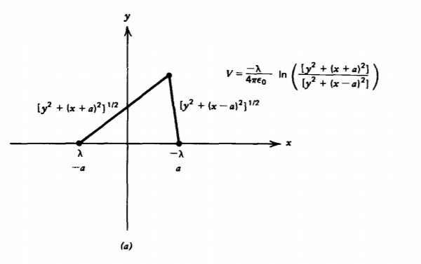
If we have two line charges of opposite polarity \(\pm \lambda\) a distance 2a apart, we choose our origin halfway between, as in Figure 2-24a, so that the potential due to both charges is just the superposition of potentials of (1):

\[V = - \frac{\lambda}{2 \pi \varepsilon_{0}} \ln \left(\frac{y^{2} + (x + a)^{2}}{y^{2} + (x-a)^{2}}\right)^{1/2} \]

where the reference potential point r_o cancels out and we use Cartesian coordinates. Equipotential lines are then

\[\frac{y^{2} + (x + a)^{2}}{y^{2} + (x-a)^{2}} = e^{-4 \pi \varepsilon_{0} V/\lambda} = K_{1} \]

where K₁ is a constant on an equipotential line. This relation is rewritten by completing the squares as

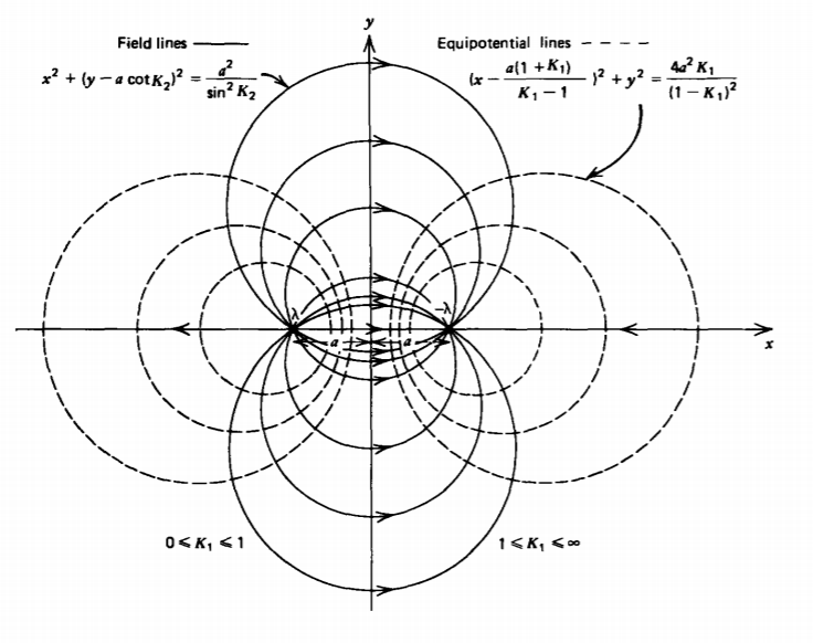
\[(x - \frac{a(1 +K_{1})}{K_{1} -1})^{2} + y^{2} = \frac{4 K_{1}a^{2}}{(1-K_{1})^{2}} \]

which we recognize as circles of radius \(r = 2a \sqrt{K_{1}}/ \vert 1 - K_{1} \vert \) with centers at y=0, x=a(1+K₁)/(K₁-1), as drawn by dashed lines in Figure 2-24b. The value of K₁ = 1 is a circle of infinite radius with center at \(x = \pm \infty\) and thus represents the x=0 plane. For values of K₁ in the interval \(0 \leq K_{1} \leq 1\) the equipotential circles are in the left half-plane, while for \(1 \leq K_{1} \leq \infty\) the circles are in the right half-plane.

The electric field is found from (2) as

\[\textbf{E} = - \nabla V = \frac{\lambda}{2 \pi \varepsilon_{0}} (\frac{-4 a x y \textbf{i}_{y} + 2a(y^{2} + a^{2} - x^{2})\textbf{i}_{x}}{[y^{2} + (x + a)^{2}][y^{2} + (x-a)^{2}]}) \]

One way to plot the electric field distribution graphically is by drawing lines that are everywhere tangent to the electric field, called field lines or lines of force. These lines are everywhere perpendicular to the equipotential surfaces and tell us the direction of the electric field. The magnitude is proportional to the density of lines. For a single line charge, the field lines emanate radially. The situation is more complicated for the two line charges of opposite polarity in Figure 2-24 with the field lines always starting on the positive charge and terminating on the negative charge.

Figure 2-24 (a) Two parallel line charges of opposite polarity a distance 2a apart. (b) The equipotential (dashed) and field (solid) lines form a set of orthogonal circles.

For the field given by (5), the equation for the lines tangent to the electric field is

\[\frac{dy}{dx} = \frac{E_{y}}{E_{x}} = -\frac{2xy}{y^{2} + a^{2} - x^{2}} \Rightarrow \frac{d(x^{2} + y^{2})}{a^{2} - (x^{2} + y^{2})} + d(\ln y) = 0 \]

where the last equality is written this way so the expression can be directly integrated to

\[x^{2} + (y-a \cot K_{2})^{2} = \frac{a^{2}}{\sin^{2} K_{2}} \]

where K₂ is a constant determined by specifying a single coordinate (x_o, y_o) along the field line of interest. The field lines are also circles of radius \(a/\sin K_{2}\) with centers at x=0, \(y = a \cot K_{2}\) as drawn by the solid lines in Figure 2-24b.

Method of Images

(a) General properties

When a conductor is in the vicinity of some charge, a surface charge distribution is induced on the conductor in order to terminate the electric field, as the field within the equipotential surface is zero. This induced charge distribution itself then contributes to the external electric field subject to the boundary condition that the conductor is an equipotential surface so that the electric field terminates perpendicularly to the surface. In general, the solution is difficult to obtain because the surface charge distribution cannot be known until the field is known so that we can use the boundary condition of Section 2.4.6. However, the field solution cannot be found until the surface charge distribution is known.

However, for a few simple geometries, the field solution can be found by replacing the conducting surface by equivalent charges within the conducting body, called images, that guarantee that all boundary conditions are satisfied. Once the image charges are known, the problem is solved as if the conductor were not present but with a charge distribution composed of the original charges plus the image charges.

(b) Line Charge Near a Conducting Plane

The method of images can adapt a known solution to a new problem by replacing conducting bodies with an equivalent charge. For instance, we see in Figure 2-24b that the field lines are all perpendicular to the x =0 plane. If a conductor were placed along the x = 0 plane with a single line charge \(\lambda\) at x = -a, the potential and electric field for x <0 is the same as given by (2) and (5).

A surface charge distribution is induced on the conducting plane in order to terminate the incident electric field as the field must be zero inside the conductor. This induced surface charge distribution itself then contributes to the external electric field for x <0 in exactly the same way as for a single image line charge \(-\lambda\)-at x =+a

The force per unit length on the line charge \(\lambda\) is due only to the field from the image charge -\(\lambda\);

\[\textbf{f} = \lambda \textbf{E} (-a, 0) = \frac{\lambda^{2}}{2 \pi \varepsilon_{0}(2a)} \textbf{i}_{x} = \frac{\lambda^{2}}{4 \pi \varepsilon_{0}a} \textbf{i}_{x} \]

From Section 2.4.6 we know that the surface charge distribution on the plane is given by the discontinuity in normal component of electric field:

\[\sigma(x = 0) = - \varepsilon_{0}E_{x}(x=0) = \frac{- \lambda a}{\pi (y^{2} + a^{2})} \]

where we recognize that the field within the conductor is zero. The total charge per unit length on the plane is obtained by integrating (9) over the whole plane:

\[\lambda_{T} = \int_{- \infty}^{+ \infty} \sigma (x = 0) dy \\ = -\frac{\lambda a}{\pi} \int_{- \infty}^{+ \infty} \frac{dy}{y^{2} +a^{2}} \\ = - \frac{\lambda a}{\pi} \frac{1}{a} \tan^{-1} \frac{y}{a} \bigg|_{- \infty}^{+ \infty} \\ = - \lambda \]

and just equals the image charge.

Line Charge and Cylinder

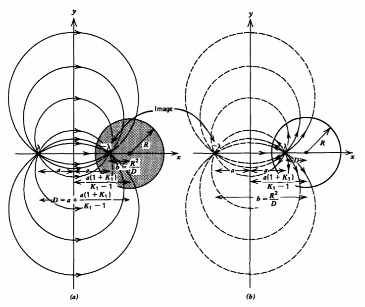
Because the equipotential surfaces of (4) are cylinders, the method of images also works with a line charge \(\lambda\) a distance D from the center of a conducting cylinder of radius R as in Figure 2-25. Then the radius R and distance a must fit (4) as

\[R = \frac{2a \sqrt{K_{1}}}{\vert 1 - K_{1} \vert}, \: \: \: \: \pm a + \frac{a (1 + K_{1})}{K_{1} - 1} = D \]

where the upper positive sign is used when the line charge is outside the cylinder, as in Figure 2-25a, while the lower negative sign is used when the line charge is within the cylinder, as in Figure 2-25b. Because the cylinder is chosen to be in the right half-plane, \(1 \leq K_{1} \leq \infty\), the unknown parameters K₁

Figure 2-25 The electric field surrounding a line charge \(\lambda\) a distance D from the center of a conducting cylinder of radius R is the same as if the cylinder were replaced by an image charge \(-\lambda\), a distance \(b = R^{2}/D\) from the center. (a) Line charge outside cylinder. (b) Line charge inside cylinder.

and a are expressed in terms of the given values R and D from (11) as

\[K_{1} = (\frac{D^{2}}{R^{2}})^{\pm 1} , \: \: \: a = \pm \frac{D^{2} - R^{2}}{2D} \]

For either case, the image line charge then lies a distance b from the center of the cylinder:

\[b = \frac{a(1 + K_{1})}{K_{1} - 1} \pm a = \frac{R^{2}}{D} \]

being inside the cylinder when the inducing charge is outside (R < D), and vice versa, being outside the cylinder when the inducing charge is inside (R >D).

The force per unit length on the cylinder is then just due to the force on the image charge:

\[F_{x} = - \frac{\lambda^{2}}{2 \pi \varepsilon_{0}(D-b)} = - \frac{\lambda^{2}D}{2 \pi \varepsilon_{0}(D^{2} - R^{2})} \]

 Wire Line

(a) Image Charges

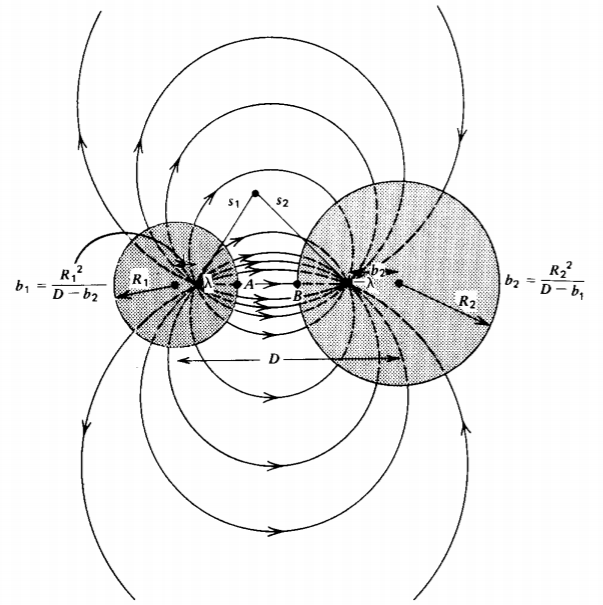
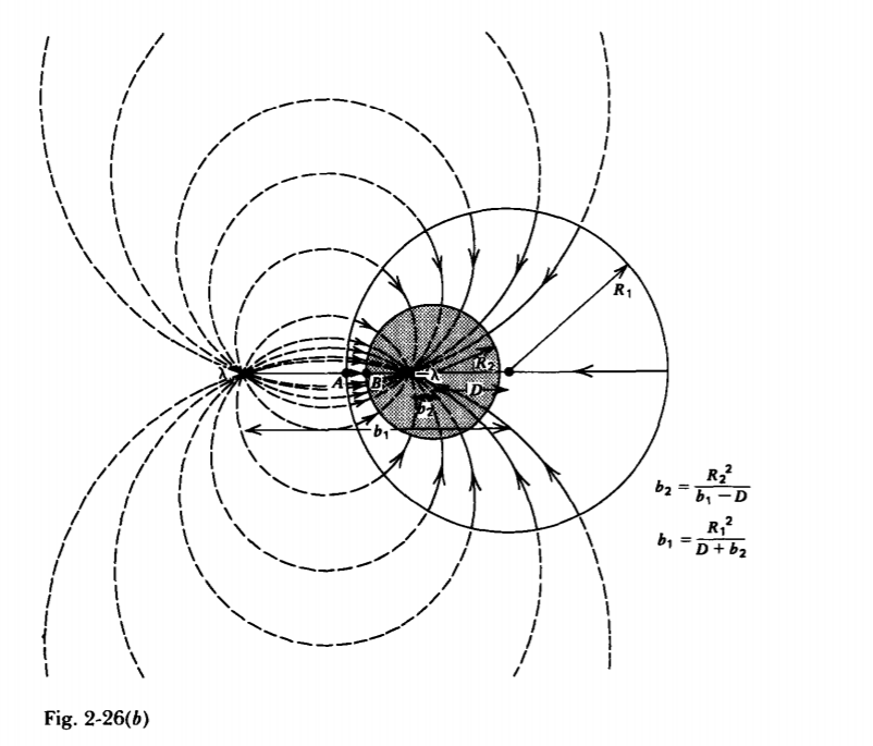
We can continue to use the method of images for the case of two parallel equipotential cylinders of differing radii R₁ and R₂ having their centers a distance D apart as in Figure 2-26. We place a line charge \(\lambda\) a distance b₁ from the center of cylinder 1 and a line charge \(-\lambda\) a distance b₂ from the center of cylinder 2, both line charges along the line joining the centers of the cylinders. We simultaneously treat the cases where the cylinders are adjacent, as in Figure 2-26a, or where the smaller cylinder is inside the larger one, as in Figure 2-26b.

The position of the image charges can be found using (13) realizing that the distance from each image charge to the center of the opposite cylinder is D - b so that

\[b_{1} = \frac{R_{1}^{2}}{D \mp b_{2}}, \: \: \: b_{2} = \pm \frac{R_{2}^{2}}{D-b_{1}} \]

where the upper signs are used when the cylinders are adjacent and lower signs are used when the smaller cylinder is inside the larger one. We separate the two coupled equations in (15) into two quadratic equations in b₁ and b₂:

\[b_{1}^{2} - \frac{[D^{2} - R_{2}^{2} + R_{1}^{2}]}{D} b_{1} + R_{1}^{2} = 0 \\ b_{2}^{2} \mp \frac{[D^{2} - R_{1}^{2} + R_{2}^{2}]}{D} b_{2} + R_{2}^{2} = 0 \]

with resulting solutions

\[b_{2} = \pm \frac{[D^{2} - R_{1}^{2} + R_{2}^{2}]}{2D} - [(\frac{D^{2} - R_{1}^{2} + R_{2}^{2}}{2D})^{2} - R_{2}^{2}]^{1/2} \\ b_{1} = \frac{[D^{2} + R_{1}^{2} - R_{2}^{2}]}{2D} \mp [({D^{2} + R_{1}^{2} - R_{2}^{2}}{2D})^{2} - R_{1}^{2}]^{1/2} \]

We were careful to pick the roots that lay outside the region between cylinders. If the equal magnitude but opposite polarity image line charges are located at these positions, the cylindrical surfaces are at a constant potential.

Figure 2-26 The solution for the electric field between two parallel conducting cylinders is found by replacing the cylinders by their image charges. The surface charge density is largest where the cylinder surfaces are closest together. This is called the proximity effect. (a) Adjacent cylinders. (b) Smaller cylinder inside the larger one.

(b) Force of Attraction

The attractive force per unit length on cylinder 1 is the force on the image charge \(\lambda\) due to the field from the opposite image charge \(-\lambda\):

\[f_{x} = \frac{\lambda^{2}}{2 \pi \varepsilon_{0}[\pm (D-b_{1})-b_{2}]} \\ = \frac{\lambda^{2}}{4 \pi \varepsilon_{0}[(\frac{D^{2} - R_{1}^{2} + R_{2}^{2}}{2D})^{2} - R_{2}^{2}]^{1/2}} \\ = \frac{\lambda^{2}}{4 \pi \varepsilon_{0} [(\frac{D^{2} - R_{2}^{2} + R_{1}^{2}}{2D})^{2} - R_{1}^{2}]^{1/2}} \]

(c) Capacitance Per Unit Length

The potential of (2) in the region between the two cylinders depends on the distances from any point to the line charges:

\[V = - \frac{\lambda}{2 \pi \varepsilon_{0}} \ln \frac{s_{1}}{s_{2}} \]

To find the voltage difference between the cylinders we pick the most convenient points labeled A and B in Figure 2-26:

\[\left. \begin{matrix} A & B \\ s_{1} = \pm (R_{1} - b_{1}) & s_{1} = \pm (D- b_{1} \mp R_{2}) \\ s_{2} = \pm (D \mp b_{2} - R_{1}) & s_{2} = R_{2} - b_{2} \end{matrix} \right. \]

although any two points on the surfaces could have been used. The voltage difference is then
\[
V_1-V_2=-\frac{\lambda}{2 \pi \varepsilon_0} \ln \left( \pm \frac{\left(R_1-b_1\right)\left(R_2-b_2\right)}{\left(D \mp b_2-R_1\right)\left(D-b_1 \mp R_2\right)}\right)
\]

This expression can be greatly reduced using the relations

\[D \mp b_{2} = \frac{R_{1}^{2}}{b_{1}}, \: \: \: \: D- b_{1} = \pm \frac{R_{2}^{2}}{b_{2}} \]

to

\[V_{1} - V_{2} = - \frac{\lambda}{2 \pi \varepsilon_{0}} \ln \frac{b_{1}b_{2}}{R_{1}R_{2}} \\ = \frac{\lambda}{2 \pi \varepsilon_{0}} \ln \left \{ \begin{matrix} \pm \frac{[D^{2} - R_{1}^{2} - R_{2}^{2}]}{2 R_{1}R_{2}} \end{matrix} \right. \\ \left. \begin{matrix} + [(\frac{D^{2} - R_{1}^{2} - R_{2}^{2}}{2R_{1}R_{2}})^{2} - 1]^{1/2} \end{matrix} \right \} \]

The potential difference \(V_{1} V_{2}\) is linearly related to the line charge A through a factor that only depends on the geometry of the conductors. This factor is defined as the capacitance per unit length and is the ratio of charge per unit length to potential difference:

\[C = \frac{\lambda}{V_{1}-V_{2}} = \frac{2 \pi \varepsilon_{0}}{ln \left \{ \begin{matrix} \pm \frac{[D^{2} - R_{1}^{2} = R_{2}^{2}]}{2 R_{1}R_{2}} + [(\frac{D^{2} - R_{1}^{2} -R_{2}^{2}}{2 R_{1}R_{2}})^{2} -1]^{1/2} \end{matrix} \right \} } \\ = \frac{2 \pi \varepsilon_{0}}{\cosh^{-1} (\pm \frac{D^{2} - R_{1}^{2} - R_{2}^{2}}{2R_{1}R_{2}})} \]

where we use the identity*

\[\ln [y + (y^{2} - 1)^{1/2}] = \cosh^{-1}y \]

*(y = \cosh x = \frac{e^{x} = e^{-x}}{2} \\ (e^{x})^{2} - 2ye^{x} + 1 = 0 \\ e^{x} = y \pm (y^{2} - 1)^{1/2} \\ x = \cosh^{-1} y = \ln[y \pm (y^{2}- 1)^{1/2}]\)

We can examine this result in various simple limits. Consider first the case for adjacent cylinders (D > R₁ + R₂ ).

1. If the distance D is much larger than the radii,

\[\lim_{D >> (R_{1} + R_{2})} C \approx \frac{2 \pi \varepsilon_{0}}{\ln [D^{2}/(R_{1}R_{2})]} = \frac{2 \pi \varepsilon_{0}}{\cosh^{-1} [D^{2}/(2 R_{1}R_{2})]} \]

2. The capacitance between a cylinder and an infinite plane can be obtained by letting one cylinder have infinite radius but keeping finite the closest distance s = D-RI-R 2 between cylinders. If we let R₁ become infinite, the capacitance becomes

\[\lim_{R_{1} \rightarrow \infty \\ D- R_{1} - R_{2} = s \textrm{ (finite)}} C = \frac{2 \pi \varepsilon_{0}}{\ln \left \{ \begin{matrix} \frac{s + R_{2}}{R_{2}} + [(\frac{s + R_{2}}{R_{2}})^{2} -1]^{1/2} \end{matrix} \right \}} \\ = \frac{2 \pi \varepsilon_{0}}{\cosh^{-1} (\frac{s + R_{2}}{R_{2}})} \]

3. If the cylinders are identical so that \(R_{1} = R_{2} = R\), the capacitance per unit length reduces to

\[\lim_{R_{1} = R_{2} = R} C = \frac{\pi \varepsilon_{0}}{\ln \left \{ \begin{matrix} \frac{D}{2R} + [(\frac{D}{2R})^{2} - 1]^{1/2} \end{matrix} \right \} } = \frac{\pi \varepsilon_{0}}{\cosh^{-1} \frac{D}{2R}} \]

4. When the cylinders are concentric so that D=0, the capacitance per unit length is

\[\lim_{D = 0} C = \frac{2 \pi \varepsilon_{0}}{\ln (R_{1}/R_{2})} = \frac{2 \pi \varepsilon_{0}}{\cosh^{-1}[(R_{1}^{2} + R_{2}^{2})/(2R_{1}R_{2})]} \]