2.7: The Method of Images with Point Charges and Spheres

Point Charge and a Grounded Sphere

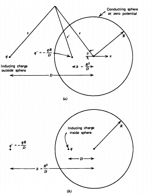
A point charge q is a distance D from the center of the conducting sphere of radius R at zero potential as shown in Figure 2-27a. We try to use the method of images by placing a single image charge q' a distance b from the sphere center along the line joining the center to the point charge q.

We need to find values of q' and b that satisfy the zero potential boundary condition at r = R. The potential at any point P outside the sphere is

\[V= \frac{1}{4 \pi \varepsilon_{0}}(\frac{q}{s} + {q'}{s'}) \]

where the distance from P to the point charges are obtained from the law of cosines:

\[s = [r^{2} + D^{2} - 2rD \cos \theta]^{1/2} \\ s' = [b^{2} + r^{2} - 2rb \cos \theta]^{1/2} \]

Figure 2-27 (a) The field due to a point charge q, a distance D outside a conducting sphere of radius R, can be found by placing a single image charge -qR/D at a distance \(b = R^{2}/D\) from the center of the sphere. (b) The same relations hold true if the charge q is inside the sphere but now the image charge is outside the sphere, since D < R.

At r = R, the potential in (1) must be zero so that q and q' must be of opposite polarity:

\[(\frac{q}{s} + \frac{q'}{s'})_{\vert_{r = R}} = 0 \Rightarrow (\frac{q}{s})^{2} + (\frac{q'}{s'})^{2}_{\vert_{r = R}} \]

where we square the equalities in (3) to remove the square roots when substituting (2),

\[q^{2}[b^{2} + R^{2} - 2Rb \cos \theta] = q'^{2}[R^{2} + D^{2} - 2RD \cos \theta] \]

Since (4) must be true for all values of \(\theta\), we obtain the following two equalities:

\[q^{2}(b^{2} + R^{2}) = q'^{2}(R^{2} + D^{2}) \\ q^{2}b = q'^{2}D \]

Eliminating q and q' yields a quadratic equation in b:

\[b^{2} - bD[1 + (\frac{R}{D})^{2}] + R^{2} = 0 \]

with solution

\[b = \frac{D}{2} [1 + (\frac{R}{D})^{2}] \pm \sqrt{\left \{ \begin{matrix} \frac{D}{2}[1 + (\frac{R}{D})^{2}] \end{matrix} \right \}^{2} - R^{2}} \\ = \frac{D}{2} [1 + (\frac{R}{D})^{2}] \pm \sqrt{\left \{ \begin{matrix} \frac{D}{2}[1 - (\frac{R}{D})^{2}] \end{matrix} \right \}^{2}} \\ = \frac{D}{2} \left \{ \begin{matrix} [1 + (\frac{R}{D})^{2}] \pm [1 - (\frac{R}{D})^{2}] \end{matrix} \right \} \]

We take the lower negative root so that the image charge is inside the sphere with value obtained from using (7) in (5):

\[b = \frac{R^{2}}{D}, \: \: \: \: q'= -q \frac{R}{D} \]

remembering from (3) that q and q' have opposite sign. We ignore the b = D solution with q'= -q since the image charge must always be outside the region of interest. If we allowed this solution, the net charge at the position of the inducing charge is zero, contrary to our statement that the net charge is q.

The image charge distance b obeys a similar relation as was found for line charges and cylinders in Section 2.6.3. Now, however, the image charge magnitude does not equal the magnitude of the inducing charge because not all the lines of force terminate on the sphere. Some of the field lines emanating from q go around the sphere and terminate at infinity.

The force on the grounded sphere is then just the force on the image charge -q' due to the field from q:

\[f_{x} = \frac{qq'}{4 \pi \varepsilon_{0}(D-b)^{2}} = - \frac{q^{2}R}{4 \pi \varepsilon_{0}D(D-b)^{2}} = - \frac{q^{2}RD}{4 \pi \varepsilon_{0}(D^{2}-R^{2})^{2}} \]

The electric field outside the sphere is found from (1) using (2) as

\[\textbf{E} = - \nabla V = \frac{1}{4 \pi \varepsilon_{0}} (\frac{q}{s^{3}} [ (r-D \cos \theta) \textbf{i}_{r} + D \sin \theta \textbf{i}_{\theta}] \\ + \frac{q'}{s'^{3}} [ (r-b) \cos \theta) \textbf{i}_{r} + b \sin \theta \textbf{i}_{\theta}]) \]

On the sphere where \(s' = (R/D)s\), the surface charge distribution is found from the discontinuity in normal electric field as given in Section 2.4.6:

\[\sigma (r=R) = \varepsilon_{0}E_{r}(r=R) = - \frac{q (D^{2} - R^{2})}{4 \pi R [ R^{2} + D^{2} - 2RD \cos \theta]^{3/2}} \]

The total charge on the sphere

\[q_{T} = \int_{0}^{\pi} \sigma(r = R) 2 \pi R^{2} \sin \theta d \theta \\ = - \frac{q}{2}R(D^{2} - R^{2}) \int_{0}^{\pi} \frac{\sin \theta d \theta }{[R^{2} + D^{2} - 2RD - \cos \theta]^{3/2}} \]

can be evaluated by introducing the change of variable

\[u = R^{2} + D^{2} - 2RD \cos \theta, \: \: \: du = 2 RD \sin \theta d \theta \]

so that (12) integrates to

\[q_{T} = - \frac{q (D^{2}-R^{2})}{4D} \int-{(D-R)^{2}}^{(D+R)^{2}} \frac{du}{u^{3/2}} = - \frac{q(D^{2}-R^{2})}{4D} (-\frac{2}{u^{1/2}}) \bigg|_{(D-R)^{2}}^{(D+R)^{2}} = - \frac{qR}{D} \]

which just equals the image charge q'.

If the point charge q is inside the grounded sphere, the image charge and its position are still given by (8), as illustrated in Figure 2-27b. Since D < R, the image charge is now outside the sphere.

Point Charge Near a Grounded Plane

If the point charge is a distance a from a grounded plane, as in Figure 2-28a, we consider the plane to be a sphere of infinite radius R so that D = R + a. In the limit as R becomes infinite, (8) becomes

\[\lim_{R \rightarrow \infty \\ D = R + a} q' = -q, \: \: \: b = \frac{R}{(1 + a/R)} = R-a \]

Figure 2-28 (a) A point charge q near a conducting plane has its image charge -q symmetrically located behind the plane. (b) An applied uniform electric field causes a uniform surface charge distribution on the conducting plane. Any injected charge must overcome the restoring force due to its image in order to leave the electrode.

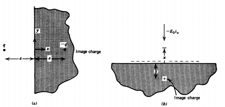
so that the image charge is of equal magnitude but opposite polarity and symmetrically located on the opposite side of the plane.

The potential at any point (x, y, z) outside the conductor is given in Cartesian coordinates as

\[V = \frac{Q}{4 \pi \varepsilon_{0}}(\frac{1}{[(x + a)^{2} + y^{2} + z^{2}]^{1/2}} - \frac{1}{[(x-a)^{2} + y^{2}+ z^{2}]^{1/2}}) \]

with associated electric field

\[\textbf{E} = - \nabla V = \frac{q}{4 \pi \varepsilon_{0}} ( \frac{(x + a)\textbf{i}_{x} + y \textbf{i}_{y} + z \textbf{i}_{z}}{[(x+a)^{2} + y^{2} + z^{2}]^{3/2}} - \frac{(x-a) \textbf{i}_{x} + y \textbf{i}_{y} + z \textbf{i}_{z}}{[(x-a)^{2} + y^{2} + z^{2}]^{3/2}}) \]

Note that as required the field is purely normal to the grounded plane

\[E_{y} (x=0) = 0, \: \: \: E_{z} (x=0) = 0 \]

The surface charge density on the conductor is given by the discontinuity of normal E:

\[\sigma(x = 0) = - \varepsilon_{0}E_{x}(x = 0) \\ = - \frac{q}{4\pi} \frac{2a}{[y^{2} + z^{2} + a^{2}]^{3/2}} \\ = - \frac{qa}{2 \pi (\textrm{r}^{2} + a^{2})^{3/2}} ; \textrm{r}^{2} = y^{2} + z^{2} \]

where the minus sign arises because the surface normal points in the negative x direction.

The total charge on the conducting surface is obtained by integrating (19) over the whole surface:

\[q_{T} = \int_{0}^{\infty} \sigma (x = 0 )2 \pi \textrm{r} d \textrm{r} \\ = - qa \int_{0}^{\infty} \frac{\textrm{r} d \textrm{r}}{(\textrm{r}^{2} + a^{2})^{3/2}} \\ = \frac{qa}{(\textrm{r}^{2} + a^{2})^{1/2}} \bigg|_{0}^{\infty} = -q \]

As is always the case, the total charge on a conducting surface must equal the image charge.

The force on the conductor is then due only to the field from the image charge:

\[\textbf{f} = - \frac{q^{2}}{16 \pi \varepsilon_{0}a^{2}} \textbf{i}_{x} \]

This attractive force prevents charges from escaping from an electrode surface when an electric field is applied. Assume that an electric field \(-E_{0} \textbf{i}_{x}\). is applied perpendicular to the electrode shown in Figure (2-28b). A uniform negative surface charge distribution \(\sigma = - \varepsilon_{0}E_{0}\) as given in (2.4.6) arises to terminate the electric field as there is no electric field within the conductor. There is then an upwards Coulombic force on the surface charge, so why aren't the electrons pulled out of the electrode? Imagine an ejected charge -q a distance x from the conductor. From (15) we know that an image charge +q then appears at -x which tends to pull the charge -q back to the electrode with a force given by (21) with a = x in opposition to the imposed field that tends to pull the charge away from the electrode. The total force on the charge -q is then

\[f_{x} = qE_{0} - \frac{q^{2}}{4 \pi \varepsilon_{0}(2x)^{2}} \]

The force is zero at position x_c

\[f_{x} = 0 \Rightarrow x_{c} = [\frac{q}{16 \pi \varepsilon_{0}E_{0}}]^{1/2} \]

For an electron (q= 1.6 x 10^-19 coulombs) in a field of \(E_{0} = 10^{6} v/m\), \(x_{c} \approx 1.9 \times 10^{-8}\) m. For smaller values of x the net force is negative tending to pull the charge back to the electrode. If the charge can be propelled past x_c by external forces, the imposed field will then carry the charge away from the electrode. If this external force is due to heating of the electrode, the process is called thermionic emission. High field emission even with a cold electrode occurs when the electric field E_o becomes sufficiently large (on the order of 10¹⁰ v/m) that the coulombic force overcomes the quantum mechanical binding forces holding the electrons within the electrode.

Sphere With Constant Charge

If the point charge q is outside a conducting sphere (D > R) that now carries a constant total charge Q₀, the induced charge is still \(q' = -qR/D\). Since the total charge on the sphere is Q₀, we must find another image charge that keeps the sphere an equipotential surface and has value \(Q_{0} + qR/D\). This other image charge must be placed at the center of the sphere, as in Figure 2-29a. The original charge q plus the image charge \(q' = -qR/D\) puts the sphere at zero potential. The additional image charge at the center of the sphere raises the potential of the sphere to

\[V = \frac{Q_{0} + qR/D}{4 \pi\varepsilon_{0}R} \]

The force on the sphere is now due to the field from the point charge q acting on the two image charges:

\[f_{x} = \frac{q}{4 \pi \varepsilon_{0}}(- \frac{qR}{D(D-b)^{2}} + \frac{(Q_{0} + qR/D)}{D^{2}}) = \frac{q}{4 \pi \varepsilon_{0}} (-\frac{qRD}{(D^{2}-R^{2})^{2}} + \frac{(Q_{0} + qR/D)}{D^{2}}) \]

Figure 2-29 (a) If a conducting sphere carries a constant charge Q₀ or (b) is at a constant voltage V₀, an additional image charge is needed at the sphere center when a charge q is nearby.

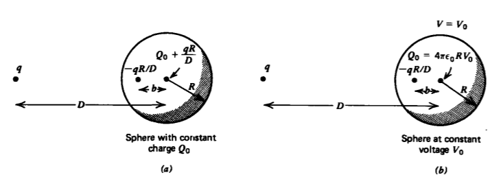
Constant Voltage Sphere

If the sphere is kept at constant voltage V₀, the image charge \(q' = -qR/D\) at distance \(b = R^{2}/D\) from the sphere center still keeps the sphere at zero potential. To raise the potential of the sphere to V₀, another image charge,

\[Q_{0} = 4 \pi \varepsilon_{0}RV_{0} \]

must be placed at the sphere center, as in Figure 2-29b. The force on the sphere is then

\[f_{x} = \frac{q}{4 \pi \varepsilon_{0}} (-\frac{qR}{D(D-b)^{2}} + \frac{Q_{0}}{D^{2}}) \]