3.1: Polarization

In many electrically insulating materials, called dielectrics, electrons are tightly bound to the nucleus. They are not mobile, but if an electric field is applied, the negative cloud of electrons can be slightly displaced from the positive nucleus, as illustrated in Figure 3-1a. The material is then said to have an electronic polarization. Orientational polarizability as in Figure 3-1b occurs in polar molecules that do not share their electrons symmetrically so that the net positive and negative charges are separated. An applied electric field then exerts a torque on the molecule that tends to align it with the field. The ions in a molecule can also undergo slight relative displacements that gives rise to ionic polarizability.

Figure 3-1 An electric dipole consists of two charges of equal magnitude but opposite sign, separated by a small vector distance d. (a) Electronic polarization arises when the average motion of the electron cloud about its nucleus is slightly displaced. (b) Orientation polarization arises when an asymmetric polar molecule tends to line up with an applied electric field. If the spacing d also changes, the molecule has ionic polarization.

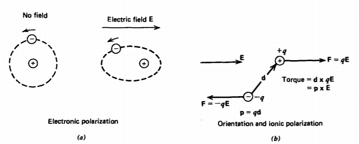
The slightly separated charges for these cases form electric dipoles. Dielectric materials have a distribution of such dipoles. Even though these materials are charge neutral because each dipole contains an equal amount of positive and negative charges, a net charge can accumulate in a region if there is a local imbalance of positive or negative dipole ends. The net polarization charge in such a region is also a source of the electric field in addition to any other free charges.

Electric Dipole

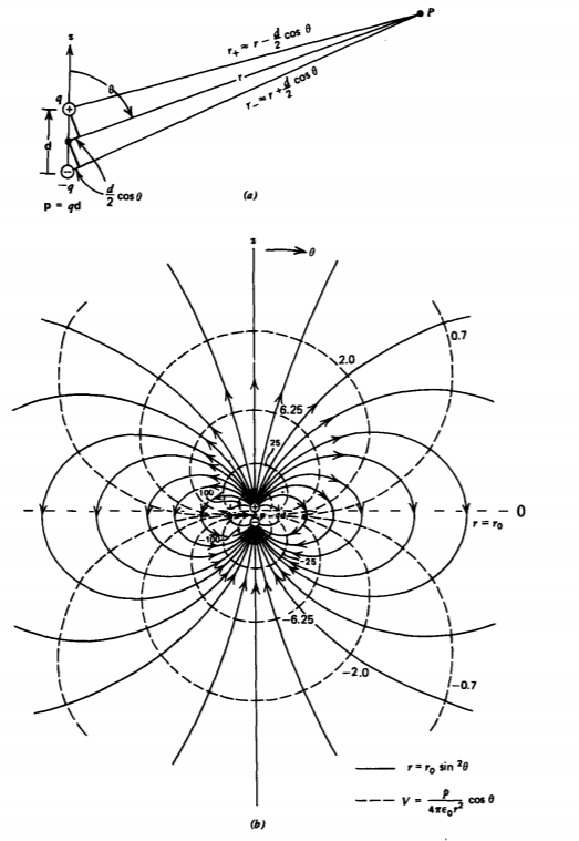
The simplest model of an electric dipole, shown in Figure 3-2a, has a positive and negative charge of equal magnitude q separated by a small vector displacement d directed from the negative to positive charge along the z axis. The electric potential is easily found at any point P as the superposition of potentials from each point charge alone:

\[V = \frac{q}{4 \pi \varepsilon_{0}r_{+}} - \frac{q}{4 \pi \varepsilon_{0}r_{-}} \]

The general potential and electric field distribution for any displacement d can be easily obtained from the geometry relating the distances r₊ and r_- to the spherical coordinates r and \(\theta\). By symmetry, these distances are independent of the angle \(\phi\). However, in dielectric materials the separation between charges are of atomic dimensions and so are very small compared to distances of interest far from the dipole. So, with r₊ and r_- much greater than the dipole spacing d, we approximate them as

\[\lim_{r>>d} \left. \begin{matrix} r_{+} \approx r - \frac{d}{2} \cos \theta \\ r_{-} \approx r + \frac{d}{2} \cos \theta \end{matrix} \right. \]

Then the potential of (1) is approximately

\[V \approx \frac{qd \cos \theta}{4 \pi \varepsilon_{0}r^{2}} = \frac{\textbf{p} \cdot \textbf{i}_{r}}{4 \pi \varepsilon_{0}r^{2}} \]

where the vector p is called the dipole moment and is defined as

\[ \textbf{p}=q \textbf{d}(\textrm{coul-m}] \]

Figure 3-2 (a) The potential at any point P due to the electric dipole is equal to the sum of potentials of each charge alone. (b) The equi-potential (dashed) and field lines (solid) for a point electric dipole calibrated for \(4 \pi \varepsilon_{0}/p = 100\).

Because the separation of atomic charges is on the order of \(1 \times 10^{-10}\, m\) with a charge magnitude equal to an integer multiple of the electron charge (q = 1.6 x 10^-19 coul), it is convenient to express dipole moments in units of debyes defined as 1 debye = 3.33 X 10^-30 coul-m so that dipole moments are of order p = 1.6 x 10^-29 coul-m \(\approx\) 4.8 debyes. The electric field for the point dipole is then

\[\textbf{E} = - \nabla V = \frac{p}{4 \pi \varepsilon_{0}r^{3}} [2 \cos \theta \textbf{i}_{r} + \sin \theta \textbf{i}_{\theta}] = \frac{3(\textbf{p} \cdot \textbf{i}_{r}) \textbf{i}_{r} - \textbf{p}}{4 \pi \varepsilon_{0}r^{3}} \]

the last expressions in (3) and (5) being coordinate independent. The potential and electric field drop off as a single higher power in r over that of a point charge because the net charge of the dipole is zero. As one gets far away from the dipole, the fields due to each charge tend to cancel. The point dipole equipotential and field lines are sketched in Figure 3-2b. The lines tangent to the electric field are

\[\frac{dr}{r d \theta} = \frac{E_{r}}{E_{\theta}} = 2 \cot \theta \Rightarrow r = r_{0} \sin^{2} \theta \]

where r₀ is the position of the field line when \(\theta = \pi/2\). All field lines start on the positive charge and terminate on the negative charge.

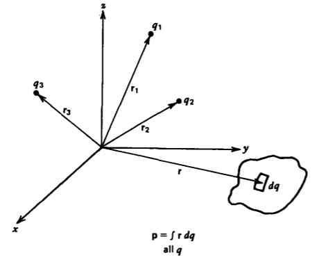
If there is more than one pair of charges, the definition of dipole moment in (4) is generalized to a sum over all charges,

\[\textbf{p} = \sum_{\textrm{all charges}} q_{i}\textbf{r}_{i} \]

where r_i is the vector distance from an origin to the charge q_i as in Figure 3-3. When the net charge in the system is zero (\(\sum q_{i} = 0\)), the dipole moment is independent of the choice of origins for if we replace r_i in (7) by r_i +r₀, where r₀ is the constant vector distance between two origins:

\[\textbf{p} = \sum q_{i} (\textbf{r}_{i} + \textbf{r}_{0}) \\ = \sum q_{i} \textbf{r}_{i} \textbf{r}_{0} \sum q_{i} \nearrow^{0} \\ = \sum q_{i} \textbf{r}_{i} \]

The result is unchanged from (7) as the constant r_o could be taken outside the summation.

If we have a continuous distribution of charge (7) is further generalized to

\[\textbf{p} = \int_{\textrm{all } q} \textbf{r} dq \]

Figure 3-3 The dipole moment can be defined for any distribution of charge. If the net charge in the system is zero, the dipole moment is independent of the location of the origin.

Then the potential and electric field far away from any dipole distribution is given by the coordinate independent expressions in (3) and (5) where the dipole moment p is given by (7) and (9).

Polarization Charge

We enclose a large number of dipoles within a dielectric medium with the differential-sized rectangular volume \(\Delta x \: \Delta y \: \Delta z\) shown in Figure 3-4a. All totally enclosed dipoles, being charge neutral, contribute no net charge within the volume. Only those dipoles within a distance \(\textbf{d} \cdot \textbf{n}\) of each surface are cut by the volume and thus contribute a net charge where n is the unit normal to the surface at each face, as in Figure 3-4b. If the number of dipoles per unit volume is N, it is convenient to define the number density of dipoles as the polarization vector P:

\[\textbf{P} = N \textbf{p} = Nq \textbf{d} \]

The net charge enclosed near surface 1 is

\[dq_{1} = (Nqd_{x})_{\vert x} \Delta y \: \Delta z = P_{x}(x) \Delta y \: \Delta z \]

while near the opposite surface 2

\[dq_{2} = - (Nqd_{x})_{\vert x + \Delta x} \Delta y \: \Delta z = - P_{x}(x + \Delta x) \: \Delta y \: \Delta z \]

Figure 3-4 (a) The net charge enclosed within a differential-sized volume of dipoles has contributions only from the dipoles that are cut by the surfaces. All totally enclosed dipoles contribute no net charge. (b) Only those dipoles within a distance \(\textbf{d} \cdot \textbf{n}\) of the surface are cut by the volume.

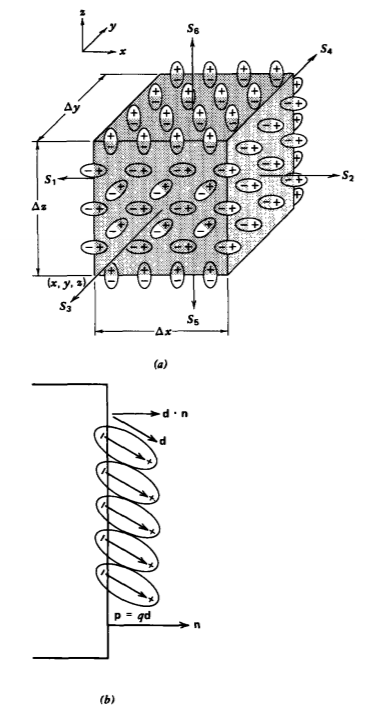
where we assume that \(\Delta y\) and \(\Delta z\) are small enough that the polarization P is essentially constant over the surface. The polarization can differ at surface 1 at coordinate x from that at surface 2 at coordinate \(x + \Delta x\) if either the number density N, the charge. q, or the displacement d is a function of x. The difference in sign between (11) and (12) is because near S₁ the positive charge is within the volume, while near S₂ negative charge remains in the volume. Note also that only the component of d normal to the surface contributes to the volume of net charge.

Similarly, near the surfaces S₃ and S₄ the net charge enclosed is

\[dq_{3} = (Nqd_{y})_{\vert y} \Delta x \: \Delta z = P_{y}(y) \Delta x \: \Delta z \\ dq_{4} = -(Nqd_{y})_{\vert y + \Delta y} \Delta x \: \Delta z = -P_{y}(y + \Delta y) \Delta x \: \Delta z \]

while near the surfaces S₅ and S₆ with normal in the z direction the net charge enclosed is

\[dq_{5} = (Nqd_{z})_{\vert z} \Delta x \: \Delta y \: = P_{z}(z)\Delta x \: \Delta y \\ dq_{6} = -(Nqd_{z})_{\vert + \Delta z} \Delta x \: \Delta y = -P_{z}(z + \Delta z) \Delta x \: \Delta y \]

The total charge enclosed within the volume is the sum of (11)-(14):

\[dq_{T} = dq_{1} + dq_{2} + dq_{3} + dq_{4} + dq_{5} + dq_{6} \\ = (\frac{P_{x}(x) - P_{x}(x + \Delta x)}{\Delta x} + \frac{P_{y}(y) - P_{y}(y + \Delta y)}{\Delta y} \\ + \frac{P_{z}(z) - P_{z}(z + \Delta z)}{\Delta z}) \Delta x \: \Delta y \: \Delta z \]

As the volume shrinks to zero size, the polarization terms in (15) define partial derivatives so that the polarization volume charge density is

\[\rho_{p} = \lim_{\Delta x \rightarrow 0 \\ \Delta y \rightarrow 0 \\ \Delta z \rightarrow 0} \frac{dq_{T}}{\Delta x \: \Delta y \: \Delta z} = -(\frac{\partial P_{x}}{\partial x} + \frac{\partial P_{y}}{\partial y} + \frac{\partial P_{z}}{\partial z}) = - \nabla \cdot \textbf{P} \]

This volume charge is also a source of the electric field and needs to be included in Gauss's law

\[\nabla \cdot (\varepsilon_{0}\textbf{E}) = \rho_{f} + \rho_{p} = \rho_{f} - \nabla \cdot \textbf{P} \]

where we subscript the free charge \(\rho_{f}\) with the letter \(f\) to distinguish it from the polarization charge \(\rho_{p}\). The total polarization charge within a region is obtained by integrating (16) over the volume,

\[q_{p} = \int_{V} \rho_{p}dV = - \int_{V} \nabla \cdot \textbf{P} dV = - \oint_{S} \textbf{P} \cdot \textbf{dS} \]

where we used the divergence theorem to relate the polarization charge to a surface integral of the polarization vector.

Displacement Field

Since we have no direct way of controlling the polarization charge, it is convenient to cast Gauss's law only in terms of free charge by defining a new vector D as

\[\textbf{D} = \varepsilon_{0} \textbf{E} + \textbf{P} \]

This vector D is called the displacement field because it differs from \(\varepsilon_{0} \textbf{E}\) due to the slight charge displacements in electric dipoles. Using (19), (17) can be rewritten as

\[\nabla \cdot (\varepsilon \textbf{E} + \textbf{P}) = \nabla \cdot \textbf{D} = \rho_{f} \]

where pf only includes the free charge and not the bound polarization charge. By integrating both sides of (20) over a volume and using the divergence theorem, the new integral form of Gauss's law is

\[\int_{V} \nabla \cdot \textbf{D} dV = \oint_{S} \textbf{D} \cdot \textbf{dS} = \int_{V} \rho_{F}dV \]

In free space, the polarization P is zero so that \(\textbf{D} = \varepsilon_{0}\textbf{E}\) and (20)-(21) reduce to the free space laws used in Chapter 2.

Linear Dielectrics

It is now necessary to find the constitutive law relating the polarization P to the applied electric field E. An accurate discussion would require the use of quantum mechanics, which is beyond the scope of this text. However, a simplified classical model can be used to help us qualitatively understand the most interesting case of a linear dielectric.

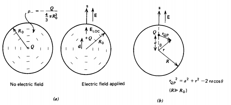
(a) Polarizability

We model the atom as a fixed positive nucleus with a surrounding uniform spherical negative electron cloud, as shown in Figure 3-5a. In the absence of an applied electric field, the dipole moment is zero because the center of charge for the electron cloud is coincident with the nucleus. More formally, we can show this using (9), picking our origin at the position of the nucleus:

\[\textbf{p} = Q(0) \nearrow^{0} - \int_{\phi = 0}^{2 \pi} \int_{\theta = 0}^{\pi} \int_{r=0}^{R_{0}} \textbf{i}_{r}\rho_{0}r^{3} \sin \theta dr \: \d \theta \: d \phi \]

Since the radial unit vector i_r changes direction in space, it is necessary to use Table 1-2 to write i_r in terms of the constant Cartesian unit vectors:

\[\textbf{i}_{r} = \sin \theta \cos \phi \textbf{i}_{x} + \sin \theta \sin \phi \textbf{i}_{y} = \cos \theta \textbf{i}_{z} \]

Figure 3-5 (a) A simple atomic classical model has a negative spherical electron cloud of small radius R₀ centered about a positive nucleus when no external electric field is present. An applied electric field tends to move the positive charge in the direction of the field and the negative charge in the opposite direction creating an electric dipole. (b) The average electric field within a large sphere of radius R (R >> R₀) enclosing many point dipoles is found by superposing the average fields due to each point charge

When (23) is used in (22) the x and y components integrate to zero when integrated over \(\phi\), while the z component is zero when integrated over \(\theta\) so that p = 0.

An applied electric field tends to push the positive charge in the direction of the field and the negative charge in the opposite direction causing a slight shift d between the center of the spherical cloud and the positive nucleus, as in Figure 3-5a. Opposing this movement is the attractive coulombic force. Considering the center of the spherical cloud as our origin, the self-electric field within the cloud is found from Section 2.4.3b as

\[E_{r} = - \frac{Qr}{4 \pi \varepsilon_{0}R_{0}^{3}} \]

In equilibrium the net force F on the positive charge is zero,

\[\textbf{F} = Q(\textbf{E}_{\textrm{Loc}} - \frac{Q\textbf{d}}{4 \pi \varepsilon_{0}R_{0}^{3}}) = 0 \]

where we evaluate (24) at r = d and E_Loc is the local polarizing electric field acting on the dipole. From (25) the equilibrium dipole spacing is

\[\textbf{d} = \frac{4 \pi \varepsilon_{0}R_{0}^{3}}{Q}\textbf{E}_{\textrm{Loc}} \]

so that the dipole moment is written as

\[\textbf{p} = Q \textbf{d} = \alpha \textbf{E}_{\textrm{Loc}}, \: \: \: \alpha = 4 \pi \varepsilon_{0}R_{0}^{3} \]

where \(\alpha\) is called the polarizability.

(b) The Local Electric Field

If this dipole were isolated, the local electric field would equal the applied macroscopic field. However, a large number density N of neighboring dipoles also contributes to the polarizing electric field. The electric field changes drastically from point to point within a small volume containing many dipoles, being equal to the superposition of fields due to each dipole given by (5). The macroscopic field is then the average field over this small volume

We calculate this average field by first finding the average field due to a single point charge Q a distance a along the z axis from the center of a spherical volume with radius R much larger than the radius of the electron cloud (R >> R₀) as in Figure 3-5b. The average field due to this charge over the spherical volume is

\[<\textbf{E}> = \frac{1}{\frac{4}{3} \pi R^{3}} \int_{r=0}^{R} \int_{\theta = 0}^{\pi} \int_{\phi=0}^{2 \pi} \frac{Q(r \textbf{i}_{r} - a \textbf{i}_{z})r^{2} \sin \theta dr \: d \theta \: d \phi}{4 \pi \varepsilon_{0}[a^{2} + r^{2} - 2 r a \: \cos \theta]^{3/2}} \]

where we used the relationships

\[r^{2}_{QP} = a^{2} + r^{2} - 2ra \cos \theta, \: \: \: \: \textbf{r}_{QP} = r \textbf{i}_{r} - a \textbf{i}_{z} \]

Using (23) in (28) again results in the x and y components being zero when integrated over \(\phi\). Only the z component is now nonzero:

\[<E_{z}> = \frac{Q}{\frac{4}{3} \pi R^{3}} \frac{2 \pi}{(4 \pi \varepsilon_{0})} \int_{\theta = 0}^{\pi} \int_{r=0}^{R} \frac{r^{3}(\cos \theta - a/r) \sin \: \theta \: dr \: d \theta}{[a^{2} + r^{2} - 2ra \: \cos \: \theta]^{3/2}} \]

We introduce the change of variable from \(\theta\) to u

\[u = r^{2} + a^{2} - 2ar \cos \theta, \: \: \: \: du = 2 ar \: \sin \theta \: d \theta \]

so that (30) can be integrated over u and r. Performing the u integration first we have

\[<E_{z}> = \frac{3Q}{8 \pi R^{3} \varepsilon_{0}} \int_{r=0}^{R} \int_{(r-a)^{2}}^{(r+a)^{2}} \frac{r}{4 a^{2}} \frac{(r^{2}-a^{2}-u)}{u^{3/2}} dr du \\ = \frac{3Q}{8 \pi R^{3} \varepsilon_{0}} \int_{r=0}^{R} \frac{r}{4a^{2}} (-\frac{2(r^{2} -a^{2} + u)}{u^{1/2}}) \bigg|_{u = (r-a)^{2}}^{(r+a)^{2}} dr \\ = - \frac{3Q}{8 \pi R^{3} \varepsilon_{0}a^{2}} \int_{r=0}^{R} r^{2}(1-\frac{r-a}{\vert r - a \vert})dr \]

We were careful to be sure to take the positive square root in the lower limit of u. Then for r >a, the integral is zero so that the integral limits over r range from 0 to a:

\[<E_{z}> = - \frac{3Q}{8 \pi R^{3} \varepsilon_{0}a^{2}} \int_{r=0}^{a} 2r^{2} dr = \frac{-Qa}{4 \pi \varepsilon_{0}R^{3}} \]

To form a dipole we add a negative charge -Q, a small distance d below the original charge. The average electric field due to the dipole is then the superposition of (33) for both charges:

\[<E_{z}> = - \frac{Q}{4 \pi \varepsilon_{0}R^{3}}[a-(a-d)] = - \frac{Qd}{4 \pi \varepsilon_{0}R^{3}} = - \frac{p}{4 \pi \varepsilon_{0}R^{3}} \]

If we have a number density N of such dipoles within the sphere, the total number of dipoles enclosed is \(\frac{4}{3} \pi R^{3}N\) so that superposition of (34) gives us the average electric field due to all the dipoles in-terms of the polarization vector P = Np:

\[<\textbf{E}> = - \frac{\frac{4}{3} \pi R^{3} N \textbf{p}}{4 \pi \varepsilon_{0} R^{3}} = - \frac{\textbf{P}}{3 \varepsilon_{0}} \]

The total macroscopic field is then the sum of the local field seen by each dipole and the average resulting field due to all the dipoles

\[ \mathbf{E}=\langle\mathbf{E}\rangle+\mathbf{E}_{\mathrm{LOC}}=-\frac{\mathbf{P}}{3 \varepsilon_0}+\mathbf{E}_{\mathrm{Loc}} \]

so that the polarization P is related to the macroscopic electric field from (27) as

\[\textbf{P} = N \textbf{p} = N \alpha \textbf{E}_{\textrm{Loc}} = N \alpha (\textbf{E} + \frac{\textbf{P}}{3 \varepsilon_{0}}) \]

which can be solved for P as

\[\textbf{P} = \frac{N \alpha}{1 - N \alpha/3 \varepsilon_{0}} \textbf{E} = \chi_{e} \varepsilon_{0} \textbf{E}, \: \: \: \chi_{e} = \frac{N \alpha /\varepsilon_{0}}{1 - N \alpha / 3 \varepsilon_{0}} \]

where we introduce the electric susceptibility \(\chi_{e}\) as the proportionality constant between P and \(\varepsilon_{0}\textbf{E}\). Then, use of (38) in (19) relates the displacement field D linearly to the electric field:

\[\textbf{D} = \varepsilon_{0} \textbf{E} + \textbf{P} = \varepsilon_{0}(1 + \chi_{e}) \textbf{E} = \varepsilon_{0} \varepsilon_{r} \text f{E} = \varepsilon \textbf{E} \]

where \(\varepsilon_{r} = 1 + \chi_{e}\) is called the relative dielectric constant and \(\varepsilon = \varepsilon_{r} \varepsilon_{0}\) is the permittivity of the dielectric, also simply called the dielectric constant. In free space the susceptibility is zero (\(\chi_{e} = 0\)) so that \(\varepsilon_{r} = 1\) and the permittivity is that of free space, \(\varepsilon = \varepsilon_{0}\). The last relation in (39) is usually the most convenient to use as all the results of Chapter 2 are also correct within

linear dielectrics if we replace \(\varepsilon_{0}\) by \(\varepsilon\). Typical values of relative permittivity are listed in Table 3-1 for various common substances. High dielectric constant materials are usually composed of highly polar molecules.

Table 3-1 The relative permittivity for various common substances at room temperature

	\(\varepsilon = \varepsilon / \varepsilon_{0}\)
Carbon Tetrachloride^a	2.2
Ethanol^a	24
Methanol^a	33
n-Hexane^a	1.9
Nitrobenzene^a	35
Pure Water^a	80
Barium Titanate^b(with 20% Strontium Titanate)	>2100
Borosilicate Glass^b	4.0
Ruby Mica (Muscovite)^b	5.4
Polyethylene^b	2.2
Polyvinyl Chloride^b	6.1
Teflon^b Polytetrafluorethylene)	2.1
Plexiglas^b	3.4
Paraffin Wax^b	2.2

^a From Lange's Handbook of Chemistry, 10th ed., McGraw-Hill, New York, 1961, pp. 1234-37.

^b From A. R. von Hippel (Ed.) Dielectric Materials and Applications, M.I.T., Cambridge, Mass., 1966, pp. 301-370

The polarizability and local electric field were only introduced so that we could relate microscopic and macroscopic fields. For most future problems we will describe materials by their permittivity \(\varepsilon\) because this constant is most easily measured. The polarizability is then easily found as

\[\varepsilon - \varepsilon_{0} = \frac{N \alpha}{1 - N \alpha/3 \varepsilon_{0}} \Rightarrow \frac{N \alpha}{3 \varepsilon_{0}} = \frac{\varepsilon - \varepsilon_{0}}{\varepsilon + 2 \varepsilon_{0}} \]

It then becomes simplest to work with the field vectors D and E. The polarization can always be obtained if needed from the definition

\[ \mathbf{P}=\mathbf{D}-\varepsilon_0 \mathbf{E}=\left(\varepsilon-\varepsilon_0\right) \mathbf{E} \]

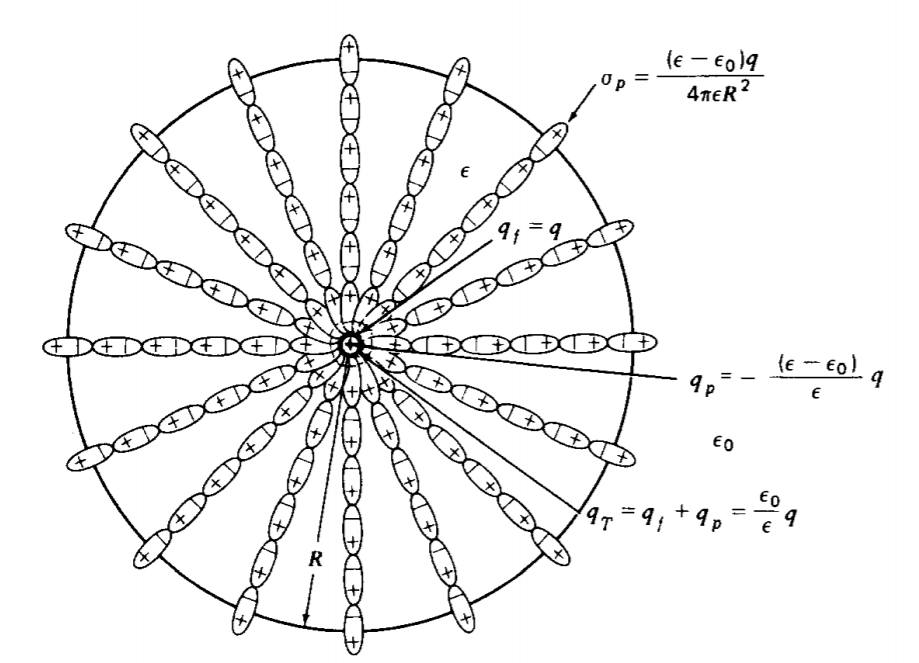
Find all the fields and charges due to a point charge q within a linear dielectric sphere of radius R and permittivity \(\varepsilon\) surrounded by free space, as in Figure 3-6.

Figure 3-6 The electric field due to a point charge within a dielectric sphere is less than the free space field because of the partial neutralization of the point charge by the accumulation of dipole ends of opposite charge. The total polarization charge on the sphere remains zero as an equal magnitude but opposite sign polarization charge appears at the spherical interface.

Answer

Applying Gauss's law of (2 1) to a sphere of any radius r whether inside or outside the sphere, the enclosed free charge is always q:

\(\oint_{S} \textbf{D} \cdot \textbf{S} = D_{r}4 \pi r^{2} = q \Rightarrow D_{r} = \frac{q}{4 \pi r^{2}} \textrm{ all } r\)

The electric field is then discontinuous at r = R,

\(E_{r} = \left \{ \begin{matrix} \frac{D_{r}}{\varepsilon} = \frac{q}{4 \pi \varepsilon r^{2} & r<R \\ \frac{D_{r}}{\varepsilon_{0}} = \frac{q}{4 \pi \varepsilon_{0}r^{2} & r>R \end{matrix} \right.\)

due to the abrupt change of permittivities. The polarization field is

\(P_{r} = D_{r} - \varepsilon_{0} E_{r} = \left \{ \begin{matrix} \frac{(\varepsilon - \varepsilon_{0})q}{4 \pi \varepsilon r^{2}}, & r < R \\ 0, & r>R \end{matrix} \right.\)

The volume polarization charge \(\rho_{P}\) is zero everywhere

\(\rho_{p} = - \nabla \cdot \textbf{P} = - \frac{1}{r^{2}} \frac{\partial}{\partial r} (r^{2} P_{r}) = 0, \: \: \: 0 < r < R\)

except at r =0 where a point polarization charge is present, and at r = R where we have a surface polarization charge found by using (18) for concentric Gaussian spheres of radius r inside and outside the dielectric sphere:

\(q_{p} = - \oint_{S} \textbf{P} \cdot \textbf{dS}= - P_{r}4 \pi r^{2} = \left \{ \begin{matrix} - (\varepsilon - \varepsilon_{0})q/\varepsilon, & r<R \\ 0 & r>R \end{matrix} \right. \)

We know that for r<R this polarization charge must be a point charge at the origin as there is no volume charge contribution yielding a total point charge at the origin:

\(Q_{T} = q_{p} + q = \frac{\varepsilon_{0}}{\varepsilon} q\)

This reduction of net charge is why the electric field within the sphere is less than the free space value. The opposite polarity ends of the dipoles are attracted to the point charge, partially neutralizing it. The total polarization charge enclosed by the sphere with r> R is zero as there is an opposite polarity surface polarization charge at r = R with density,

\(\sigma_{p} = \frac{(\varepsilon - \varepsilon_{0})q}{4 \pi \varepsilon R^{2}}\)

The total surface charge \(\sigma_{p} 4 \pi R^{2} = (\varepsilon - \varepsilon_{0}) q/\varepsilon\) is equal in magnitude but opposite in sign to the polarization point charge at the origin. The total p6larization charge always sums to zero.

Spontaneous Polarization

(a) Ferro-electrics Examining (38) we see that when \(N \alpha/3 \varepsilon_{0}=1\) the polarization can be nonzero even if the electric field is zero. We can just meet this condition using the value of polarizability in (27) for electronic polarization if the whole volume is filled with contacting dipole spheres of the type in Figure 3-5a so that we have one dipole for every volume of \(\frac{4}{3} \pi R_{0}^{3}\) Then any slight fluctuation in the local electric field increases the polarization, which in turn increases the local field resulting in spontaneous polarization so that all the dipoles over a region are aligned. In a real material dipoles are not so densely packed. Furthermore, more realistic statistical models including thermally induced motions have shown that most molecules cannot meet the conditions for spontaneous polarization.

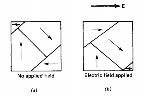
However, some materials have sufficient additional contributions to the polarizabilities due to ionic and orientational polarization that the condition for spontaneous polarization is met. Such materials are called ferro-electrics, even though they are not iron compounds, because of their similarity in behavior to iron compound ferro-magnetic materials, which we discuss in Section 5.5.3c. Ferro-electrics are composed of permanently polarized regions, called domains, as illustrated in Figure 3-7a. In the absence of an electric field, these domains are randomly distributed so that the net macroscopic polarization field is zero. When an electric field is applied, the dipoles tend to align with the field so that domains with a polarization component along the field grow at the expense of nonaligned domains. Ferro-electrics typically have very high permittivities such as barium titanate listed in Table 3-1.

The domains do not respond directly with the electric field as domain orientation and growth is not a reversible process but involves losses. The polarization P is then nonlinearly related to the electric field E by the hysteresis curve shown in Figure 3-8. The polarization of an initially unpolarized sample increases with electric field in a nonlinear way until the saturation value P_sat is reached when all the domains are completely aligned with the field. A further increase in E does not increase P as all the dipoles are completely aligned.

As the field decreases, the polarization does not retrace its path but follows a new path as the dipoles tend to stick to their previous positions. Even when the electric field is zero, a

Figure 3-7 (a) In the absence of an applied electric field, a ferro-electric material generally has randomly distributed permanently polarized domains. Over a macroscopic volume, the net polarization due to all the domains is zero. (b) When an electric field is applied, domains with a polarization component in the direction of the field grow at the expense of nonaligned domains so that a net polarization can result.

Figure 3-8 A typical ferro-electric hysteresis curve shows a saturation value P_sat when all the domains align with the field, a remanent polarization P_r when the electric field is removed, and a negative coercive electric field - E_c, necessary to bring the polarization back to zero.

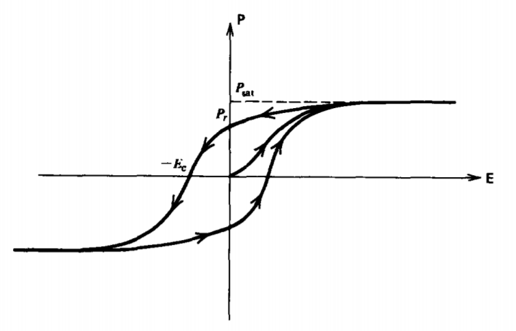
remanent polarization P_r remains. To bring the polarization to zero requires a negative coercive field -E_c. Further magnitude increases in negative electric field continues the symmetric hysteresis loop until a negative saturation is reached where all the dipoles have flipped over. If the field is now brought to zero and continued to positive field values, the whole hysteresis curve is traversed.

(b) Electrets

There are a class of materials called electrets that also exhibit a permanent polarization even in the absence of an applied electric field. Electrets are typically made using certain waxes or plastics that are heated until they become soft. They are placed within an electric field, tending to align the dipoles in the same direction as the electric field, and then allowed to harden. The dipoles are then frozen in place so that even when the electric field is removed a permanent polarization remains.

Other interesting polarization phenomena are:

Electrostriction- slight change in size of a dielectric due to the electrical force on the dipoles.

Piezo-electricity- when the electrostrictive effect is reversible so that a mechanical strain also creates a field.

Pyro-electricity- induced polarization due to heating or cooling.