3.2: Conduction

Conservation of Charge

In contrast to dielectrics, most metals have their outermost band of electrons only weakly bound to the nucleus and are free to move in an applied electric field. In electrolytic solutions, ions of both sign are free to move. The flow of charge, called a current, is defined as the total charge flowing through a surface per unit time. In Figure 3-9a a single species of free charge with density \(\rho_{fi}\) and velocity \(\textbf{v}_{i}\) flows through a small differential sized surface dS.

Figure 3-9 The current through a surface is defined as the number of charges per second passing through the surface. (a) The current is proportional to the component of charge velocity perpendicular to the surface. (b) The net change of total charge within a volume is equal to the difference of the charge entering to that leaving in a small time \(\Delta t\).

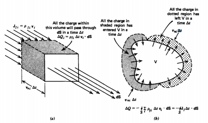
The total charge flowing through this surface in a time \(\Delta t\) depends only on the velocity component perpendicular to the surface:

\[\Delta Q_{i} = \rho_{fi} \Delta t \textbf{v}_{i} \cdot \textbf{dS} \]

The tangential component of the velocity parallel to the surface dS only results in charge flow along the surface but not through it. The total differential current through dS is then defined as

\[dI_{i} = \frac{\Delta Q_{i}}{\Delta t} = \rho_{fi}\textbf{v}_{i} \cdot \textbf{dS} = \textbf{J}_{fi} \cdot \textbf{dS} \: \textrm{ ampere} \]

where the free current density of these charges \(\textbf{J}_{fi}\) is a vector and is defined as

\[\textbf{J}_{fi} = \rho_{fi} \textbf{v}_{i} \textrm{amp/m}^{2} \]

If there is more than one type of charge carrier, the net charge density is equal to the algebraic sum of all the charge densities, while the net current density equals the vector sum of the current densities due to each carrier:

\[\rho_{f} = \sum \rho_{fi}, \: \: \textbf{J}_{f} = \sum \rho_{fi}\textbf{v}_{i} \]

Thus, even if we have charge neutrality so that \(\rho_{f} = 0\), a net current can flow if the charges move with different velocities. For example, two oppositely charged carriers with densities \(\rho_{1} = - \rho_{2} \equiv \rho_{0}\) moving with respective velocities \(\textbf{v}_{1}\) and \(\textbf{v}_{2}\) have

\[\rho_{f} = \rho_{1} + \rho_{2} = 0, \: \: \: \textbf{J}_{f} = \rho_{1} \textbf{v}_{1} + \rho_{2} \textbf{v}_{2} = \rho_{0} (\textbf{v}_{1} - \textbf{v}_{2}) \]

With \(\textbf{v}_{1} \neq \textbf{v}_{2}\) a net current flows with zero net charge. This is typical in metals where the electrons are free to flow while the oppositely charged nuclei remain stationary.

The total current I, a scalar, flowing through a macroscopic surface S, is then just the sum of the total differential currents of all the charge carriers through each incremental size surface element:

\[I = \int_{S} \textbf{J}_{f} \cdot \textbf{dS} \]

Now consider the charge flow through the closed volume V with surface S shown in Figure 3-9b. A time At later, that charge within the volume near the surface with the velocity component outward will leave the volume, while that charge just outside the volume with a velocity component inward will just enter the volume. The difference in total charge is transported by the current:

\[\Delta Q = \int_{V} [\rho_{f}(t + \Delta t) \rho_{f}(t)] \textrm{dV} \\ = - \oint_{S} \sum \rho_{fi} \textbf{v}_{i} \Delta t \cdot \textbf{dS} = - \oint_{S} \textbf{J}_{f} \Delta t \cdot \textbf{dS} \]

The minus sign on the right is necessary because when v_i is in the direction of dS, charge has left the volume so that the enclosed charge decreases. Dividing (7) through by \(\Delta t\) and taking the limit as \(\Delta t \rightarrow 0\), we use (3) to derive the integral conservation of charge equation:

\[\oint_{S} \textbf{J}_{f} \cdot \textbf{dS} + \int_{\textrm{V}} \frac{\partial \rho_{f}}{\partial t} d \textrm{V} = 0 \]

Using the divergence theorem, the surface integral can be converted to a volume integral:

\[\int_{\textrm{V}} [\nabla \cdot \textbf{J}_{f} + \frac{\partial \rho f}{\partial t}] d \textrm{V} = 0 \Rightarrow \nabla \cdot \textbf{J}_{f} + \frac{\partial \rho_{f}}{\partial t} = 0 \]

where the differential point form is obtained since the integral must be true for any volume so that the bracketed term must be zero at each point. From Gauss's law (\(\nabla \codt \textbf{D} = \rho_{f}\)) (8) and (9) can also be written as

\[\oint_{S}(\textbf{J}_{f} + \frac{\partial \textbf{D}}{\partial t}) \cdot \textbf{dS} = 0, \: \: \: \nabla \cdot (\textbf{J}_{f} + \frac{\partial \textbf{D}}{\partial t}) = 0 \]

where J_f is termed the conduction current density and \(\partial \textbf{D} / \partial t\) is called the displacement current density.

This is the field form of Kirchoff's circuit current law that the algebraic sum of currents at a node sum to zero. Equation (10) equivalently tells us that the net flux of total current, conduction plus displacement, is zero so that all the current that enters a surface must leave it. The displacement current does not involve any charge transport so that time-varying current can be transmitted through space without charge carriers. Under static conditions, the displacement current is zero.

Charged Gas Conduction Models

(a) Governing Equations. In many materials, including good conductors like metals, ionized gases, and electrolytic solutions as well as poorer conductors like lossy insulators and semiconductors, the charge carriers can be classically modeled as an ideal gas within the medium, called a plasma. We assume that we have two carriers of equal magnitude but opposite sign \(\pm q\) with respective masses \(m_{\pm}\) and number densities \(n_{\pm}\). These charges may be holes and electrons in a semiconductor, oppositely charged ions in an electrolytic solution, or electrons and nuclei in a metal. When an electric field is applied, the positive charges move in the direction of the field while the negative charges move in the opposite direction. These charges collide with the host medium at respective frequencies \(\nu_{+}\) and \(\nu_{-}\), which then act as a viscous or frictional dissipation opposing the motion. In addition to electrical and frictional forces, the particles exert a force on themselves through a pressure term due to thermal agitation that would be present even if the particles were uncharged. For an ideal gas the partial pressure p is

\[p = nkT \textrm{ pascals }[\textrm{kg s}^{-2} \cdot \textrm{m}^{-1}] \]

where n is the number density of charges, T is the absolute temperature, and \(k = 1.38 \times 10^{-23} \textrm{joule}/^{\circ}K\) is called Boltzmann's constant.

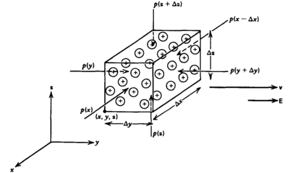
The net pressure force on the small rectangular volume shown in Figure 3-10 is

\[\textbf{f}_{p} = (\frac{p(x - \Delta x) - p (x)}{\Delta x} \textbf{i}_{x} + \frac{p(y) - p(y + \Delta y)}{\Delta y} \textbf{i}_{y} \\ + \frac{p(z) - p(z + \Delta z)}{\Delta z} \textbf{i}_{z}) \Delta x \Delta y \Delta z \]

where we see that the pressure only exerts a net force on the volume if it is different on each opposite surface. As the volume shrinks to infinitesimal size, the pressure terms in (12) define partial derivatives so that the volume force density becomes

\[\lim_{\Delta x \rightarrow 0 \\ \Delta y \rightarrow 0 \\ \Delta z \rightarrow 0} \frac{\textbf{f}_{p}}{\Delta x \Delta y \Delta z} = -(\frac{\partial p}{\partial x} \textbf{i}_{x} + \frac{\partial p}{\partial y} \textbf{i}_{y} + \frac{\partial p}{\partial z} \textbf{i}_{z}) = - \nabla p \]

Then using (11)-(13), Newton's force law for each charge carrier within the small volume is

\[m_{\pm} \frac{\partial \textbf{v}_{\pm}}{\partial t} = \pm q \textbf{E} - m_{\pm} \nu_{\pm} \textbf{v}_{\pm} - \frac{1}{n_{\pm}} \nabla (n_{\pm} kT) \]

Figure 3-10 Newton's force law, applied to a small rectangular volume \(\Delta x \: \Delta y \: \Delta z\) moving with velocity v, enclosing positive charges with number density n. The pressure is the force per unit area acting normally inward on each surface and only contributes to the net force if it is different on opposite faces.

where the electric field E is due to the imposed field plus the field generated by the charges, as given by Gauss's law.

(b) Drift-Diffusion Conduction

Because in many materials the collision frequencies are typically on the order of \(\nu \approx 10^{13} \textrm{Hz}\), the inertia terms in (14) are often negligible. In this limit we can easily solve (14) for the velocity of each carrier as

\[\lim_{\partial \textbf{v}_{\pm}/\partial t << \nu_{\pm} \textbf{v}_{\pm}} \textbf{v}_{\pm} = \frac{1}{m_{\pm} \nu_{\pm}} ( \pm q \textbf{E} - \frac{1}{n_{\pm}} \nabla (n_{\pm}kT)) \]

The charge and current density for each carrier are simply given as

\[\rho_{\pm} = \pm qn_{\pm}, \: \: \: \textbf{J}_{\pm} = \rho_{\pm}\textbf{v}_{\pm} = \pm q n_{\pm}\textbf{\pm} \]

Multiplying (15) by the charge densities then gives us the constitutive law for each current as

\[\textbf{J}_{\pm} = \pm qn_{\pm}\textbf{v}_{\pm} = \pm \rho_{\pm} \mu_{\pm}\textbf{E} - D_{\pm} \nabla \rho_{\pm} \]

where \(\mu_{\pm}\) are called the particle mobilities and \(D_{\pm}\) are their diffusion coefficients

\[\mu_{\pm} = \frac{q}{m_{\pm}\nu_{\pm}} [\textrm{A kg}^{-1} \cdot \textrm{s}^{-2}], \: \: \: D_{\pm} = \frac{kT}{m_{\pm}\nu_{pm}}[\textrm{m}^{2} \cdot \textrm{s}^{-1}] \]

assuming that the system is at constant temperature. We see that the ratio \(D_{\pm}/\mu_{\pm}\) for each carrier is the same having units of voltage, thus called the thermal voltage:

\[\frac{D_{\pm}}{\mu_{\pm}} = \frac{kT}{q} \textrm{volts} [ \textrm{kg m}^{2} \cdot \textrm{A}^{-1} \cdot \textrm{s}^{-3}] \]

This equality is known as Einstein's relation.

In equilibrium when the net current of each carrier is zero, (17) can be written in terms of the potential as (\(\textbf{E} = - \nabla V\))

\[\textbf{J}_{+} = \textbf{J}_{-} = 0 = - \rho_{\pm} \mu_{\pm} \nabla V \mp D_{\pm} \nabla \rho_{\pm} \]

which can be rewritten as

\[\nabla [\pm \frac{\mu_{\pm}}{D_{\pm}} V + \ln \rho_{\pm}]=0 \]

The bracketed term can then only be a constant, so the charge density is related to the potential by the Boltzmann distribution:

\[\rho_{\pm} = \pm \rho_{0} e^{\mp qV/kT} \]

where we use the Einstein relation of (19) and \(\pm \rho_{0}\) is the equilibrium charge density of each carrier when V=0 and are of equal magnitude because the system is initially neutral.

To find the spatial dependence of \(\rho\) and V we use (22) in Poisson's equation derived in Section 2.5.6:

\[\nabla^{2}V = - \frac{(\rho_{+} + \rho_{-})}{\varepsilon} = - \frac{\rho_{0}}{\varepsilon}(e^{-qV}{kT}-e^{qV/kT})= \frac{2 \rho_{0}}{\varepsilon} \sinh \frac{qV}{kT} \]

This equation is known as the Poisson-Boltzmann equation because the charge densities obey Boltzmann distributions.

Consider an electrode placed at x = 0 raised to the potential \(V_{0}\) with respect to a zero potential at \(x = \pm \infty\), as in Figure 3-11 a. Because the electrode is long, the potential only varies

Figure 3-11 Opposite polarity mobile charges accumulate around any net charge inserted into a conductor described by the drift-diffusion equations, and tend to shield out its field for distances larger than the Debye length. (a) Electrode at potential V_o with respect to a zero potential at \(x = \pm \infty\). The spatial decay is faster for larger values of V_o. (b) Point charge.

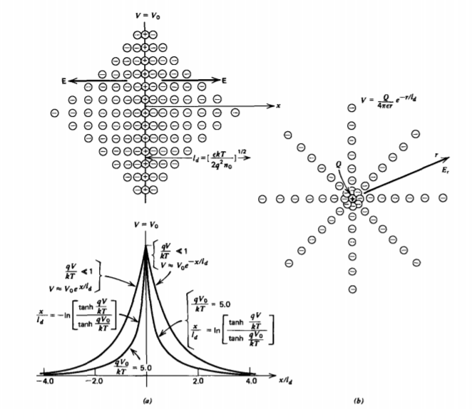
with the x coordinate so that (23) becomes

\[\frac{d^{2}\tilde{V}}{dx^{2}} - \frac{1}{l^{2}_{d}} \sinh \tilde{V} = 0, \: \: \: \tilde{V} = \frac{qV}{kT}, \: \: \: l_{d}^{2}= \frac{\varepsilon kT}{2 \rho_{0}q} \]

where we normalize the voltage to the thermal voltage kT/q and l_d is called the Debye length.

If (24) is multiplied by dV/dx, it can be written as an exact differential:

\[\frac{d}{dx}[\frac{1}{2}(\frac{d \tilde{V}}{dx})^{2} - \frac{\cosh \tilde{V}}{l_{d}^{2}}] = 0 \]

The bracketed term must then be a constant that is evaluated far from the electrode where the potential and electric field \(\tilde{E} = -d \tilde{V}/dx\) are zero:

\[\frac{d \tilde{V}}{dx} = - \tilde{E}_{x} = [\frac{2}{l^{2}_{d}} (\cosh \tilde{V} -1)]^{1/2} = \mp \frac{2}{l_{d}} \sinh \frac{\tilde{V}}{2} \left \{ \begin{matrix} x>0 \\ x<0 \end{matrix} \right. \]

The different signs taken with the square root are necessary because the electric field points in opposite directions on each side of the electrode. The potential is then implicitly found by direct integration as

\[\frac{\tanh (\tilde{V}/4)}{\tanh (\tilde{V}_{0}/4)} = e^{\mp x/l_{d}} \left \{ \begin{matrix} x>0 \\ x<0 \end{matrix} \right. \]

The Debye length thus describes the characteristic length over which the applied potential exerts influence. In many materials the number density of carriers is easily of the order of \(n_{0} \approx 10^{20}/m^{3}\), so that at room temperature (\(T \approx 293^{\circ}K\)), l_d is typically 10^-7 m.

Often the potentials are very small so that \(qv/kT<<1\). Then, the hyperbolic terms in (27), as well as in the governing equation of (23), can be approximated by their arguments:

\[\nabla^{2}V - \frac{V}{l^{2}_{d}} =0 \]

This approximation is only valid when the potentials are much less than the thermal voltage \(kt/q\), which, at room temperature is about 25 mv. In this limit the solution of (27) shows that the voltage distribution decreases exponentially. At higher values of Vo, the decay is faster, as shown in Figure 3-11 a.

If a point charge Q is inserted into the plasma medium, as in Figure 3-11 b, the potential only depends on the radial distance r. In the small potential limit, (28) in spherical coordinates is

\[\frac{1}{r^{2}} \frac{\partial}{\partial r} (r^{2} \frac{\partial V}{\partial r}) - \frac{V}{l_{d}^{2}} = 0 \]

Realizing that this equation can be rewritten as

\[\frac{\partial^{2}}{\partial r^{2}} (rV) - \frac{(rV)}{l_{d}^{2}}=0 \]

we have a linear constant coefficient differential equation in the variable (rV) for which solutions are

\[rV = A_{1} e^{-r/l_{d}}+ A_{2}e^{+r/l_{d}} \]

Because the potential must decay and not grow far from the charge, \(A_{2}=0\) and the solution is

\[V= \frac{Q}{4 \pi \varepsilon r} e^{-r/l_{d}} \]

where we evaluated \(A_{1}\) by realizing that as \(r \rightarrow 0\) the potential must approach that of an isolated point charge. Note that for small r the potential becomes very large and the small potential approximation is violated.

(c) Ohm's Law

We have seen that the mobile charges in a system described by the drift-diffusion equations accumulate near opposite polarity charge and tend to shield out its effect for distances larger than the Debye length. Because this distance is usually so much smaller than the characteristic system dimensions, most regions of space outside the Debye sheath are charge neutral with equal amounts of positive and negative charge density \(\pm \rho_{0}\). In this region, the diffusion term in (17) is negligible because there are no charge density gradients. Then the total current density is proportional to the electric field:

\[\textbf{J} = \textbf{J}_{+} + J_{-} = \rho_{0}(\textbf{v}_{+} - \textbf{v}_{-}) = qn_{0}(\mu_{+} + \mu_{-}) \textbf{E} = \sigma \textbf{E} \]

where \(\sigma\) [siemans/m (m^-3 kg^-1 s³ A²)] is called the Ohmic conductivity and (33) is the point form of Ohm's law. Sometimes it is more convenient to work with the reciprocal conductivity \(\rho_{r} = (1/\rho)\) (ohm-m) called the resistivity. We will predominantly use Ohm's law to describe most media in this text, but it is important to remember that it is often not valid within the small Debye distances near charges. When Ohm's law is valid, the net charge is zero, thus giving no contribution to Gauss's law. Table 3-2 lists the Ohmic conductivities for various materials. We see that different materials vary over wide ranges in their ability to conduct charges.

The Ohmic conductivity of "perfect conductors" is large and is idealized to be infinite. Since all physical currents in (33) must remain finite, the electric field within the conductor is zero so that it imposes an equipotential surface:

\[\lim_{\sigma \rightarrow \infty} \textbf{J} = \sigma \textbf{E} \Rightarrow \left \{ \begin{matrix} \textbf{E} = 0 \\ V = \textrm{const} \\ \textbf{J} = \textrm{finite} \end{matrix} \right. \]

Table 3-2 The Ohmic conductivity for various common substances at room temperature

	\(\sigma\) [siemen/m]
Silver^a	6.3 x 10^7
Copper^a	5.9 x 10^7
Gold^a	4.2 x 10^7
Lead^a	0.5 x 10^7
Tin^a	0.9 x 10^7
Zinc^a	1.7 x 10^7
Carbon^a	7.3 x 10^-4
Mercury^b	1.06 x 10^6
Pure Water^b	4 x 10^-6
Nitrobenzene^b	5 x 10^-7
Methanol^b	4 x 10^-5
Ethanol^b	1.3 x 10^-7
Hexane^b	<1 x 10^-18

^a From Handbook of Chemistry and Physics, 49th ed., The Chemical Rubber Co., 1968, p. E80.

^b From Lange's Handbook of Chemistry, 10th ed., McGraw-Hill, New York, 1961, pp. 1220-21.

Throughout this text electrodes are generally assumed to be perfectly conducting and thus are at a constant potential. The external electric field must then be incident perpendicularly to the surface

(d) Superconductors

One notable exception to Ohm's law is for superconducting materials at cryogenic temperatures. Then, with collisions negligible (\(\nu_{\pm} = 0\)) and the absolute temperature low (\(T \approx 0\)), the electrical force on the charges is only balanced by their inertia so that (14) becomes simply

\[\frac{\partial \textbf{V}_{\pm}}{\partial t} = \pm \frac{q}{m_{\pm}} \textbf{E} \]

We multiply (35) by the charge densities that we assume to be constant so that the constitutive law relating the current density to the electric field is

\[\frac{\partial (\pm qn_{\pm} \textbf{v}_{\pm})}{\partial t} = \frac{\partial \textbf{J}_{\pm}}{\partial t} = \frac{q^{2}n_{\pm}}{m_{\pm}} \textbf{E} = \omega^{2}_{p_{\pm}} \varepsilon \textbf{E}, \: \: \: \omega^{2}_{p_{\pm}} = \frac{q^{2}n_{pm}}{m_{\pm}\varepsilon} \]

where \(\omega_{p \pm}\) is called the plasma frequency for each carrier.

For electrons (q = -1.6 x 10^-19 coul, m_ = 9.1 x 10^-31 kg) of density \(n_{-} \approx 10^{20}/m^{3}\) within a material with the permittivity of free space, \(\varepsilon = \varepsilon_{0} \approx 8.854 \times 10^{-12}\) farad/m, the plasma frequency is

\[\omega_{p_{-}} = \sqrt{q^{2}n_{-}/m_{- \varepsilon}} \approx 5.6 \times 10^{11} \textrm{ radian/sec} \\ \Rightarrow f_{p_{-}} = \omega_{p_{-}}/2 \pi \approx 9 \times 10^{10} \textrm{Hz} \]

If such a material is placed between parallel plate electrodes that are open circuited, the electric field and current density J = J₊+J_ must be perpendicular to the electrodes, which we take as the x direction. If the electrode spacing is small compared to the width, the interelectrode fields far from the ends must then be x directed and be only a function of x. Then the time derivative of the charge conservation equation in (10) is

\[\frac{\partial}{\partial x} [ \frac{\partial}{\partial t} (J_{+} + J_{-}) + \varepsilon \frac{\partial^{2}E}{\partial t^{2}}]=0 \]

The bracketed term is just the time derivative of the total current density, which is zero because the electrodes are open circuited so that using (36) in (38) yields

\[\frac{\partial^{2}E}{\partial t^{2}} + \omega^{2}_{p} E = 0, \:\: \: \omega^{2}_{p} = \omega^{2}_{p +} + \omega^{2}_{p -} \]

which has solutions

\[E = A_{1} \sin \omega_{p}t + A_{2} \cos \omega_{p}t \]

Any initial perturbation causes an oscillatory electric field at the composite plasma frequency w,. The charges then execute simple harmonic motion about their equilibrium position.