3.3: Field Boundary Conditions

In many problems there is a surface of discontinuity separating dissimilar materials, such as between a conductor and a dielectric, or between different dielectrics. We must determine how the fields change as we cross the interface where the material properties change abruptly

Tangential Component of E

We apply the line integral of the electric field around a contour of differential size enclosing the interface between dissimilar materials, as shown in Figure 3-12a. The long sections a and c of length dl are tangential to the surface and the short joining sections b and d are of zero length as the interface is assumed to have zero thickness. Applying the line integral of the electric field around this contour, from Section 2.5.6 we obtain

\[\oint_{L} \textbf{E} \cdot \textbf{dl} = (E_{1t} - E_{2t}) dl = 0 \]

where E_1t and E_2t are the components of the electric field tangential to the interface. We get no contribution from the normal components of field along sections b and d because the contour lengths are zero. The minus sign arises along c because the electric field is in the opposite direction of the contour traversal. We thus have that the tangential

Figure 3-12 (a) Stokes' law applied to a line integral about an interface of discontinuity shows that the tangential component of electric field is continuous across the boundary. (b) Gauss's law applied to a pill-box volume straddling the interface shows that the normal component of displacement vector is discontinuous in the free surface charge density \(\sigma_{f}\).

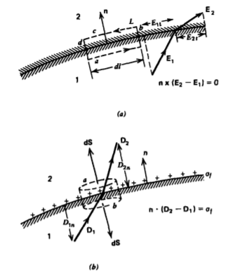
components of the electric field are continuous across the interface

\[E_{1t} = E_{2t} \Rightarrow \textbf{n} \times (\textbf{E}_{2} - \textbf{E}_{1}) =0 \]

where n is the interfacial normal shown in Figure 3-12a.

Within a perfect conductor the electric field is zero. Therefore, from (2) we know that the tangential component of E outside the conductor is also zero. Thus the electric field must always terminate perpendicularly to a perfect conductor

Normal Component of D

We generalize the results of Section 2.4.6 to include dielectric media by again choosing a small Gaussian surface whose upper and lower surfaces of area dS are parallel to a surface charged interface and are joined by an infinitely thin cylindrical surface with zero area, as shown in Figure 3-12b. Then only faces a and b contribute to Gauss's law:

\[\oint_{S} \textbf{D} \cdot \textbf{dS} = (D_{2n} -D_{1n}) d \textbf{S} = \oint_{f} d \textbf{S} \]

where the interface supports a free surface charge density \(sigma_{f}\) and \(D_{2n}\) and \(D_{1n}\) are the components of the displacement vector on either side of the interface in the direction of the normal n shown, pointing from region 1 to region 2. Reducing (3) and using more compact notation we have

\[D_{2n} -D_{1n} = \sigma_{f}, \: \: \: \textbf{n} \cdot (\textbf{D}_{2} - \textbf{D}_{1}) = \sigma_{f} \]

where the minus sign in front of D₁ arises because the normal on the lower surface b is -n. The normal components of the displacement vector are discontinuous if the interface has a surface charge density. If there is no surface charge (\(\sigma_{f} = 0\)), the normal components of D are continuous. If each medium has no polarization, (4) reduces to the free space results of Section 2.4.6.

At the interface between two different lossless dielectrics, there is usually no surface charge (\(\sigma_{f} =0\)), unless it was deliberately placed, because with no conductivity there is no current to transport charge. Then, even though the normal component of the D field is continuous, the normal component of the electric field is discontinuous because the dielectric constant in each region is different.

At the interface between different conducting materials, free surface charge may exist as the current may transport charge to the surface discontinuity. Generally for such cases, the surface charge density is nonzero. In particular, if one region is a perfect conductor with zero internal electric field, the surface charge density on the surface is just equal to the normal component of D field at the conductor's surface,

\[\sigma_{f} = \textbf{n} \cdot \textbf{D} \]

where n is the outgoing normal from the perfect conductor.

Point Charge Above a Dielectric Boundary

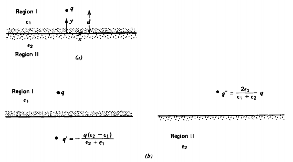
If a point charge q within a region of permittivity \(\varepsilon_{1}\) is a distance d above a planar boundary separating region I from region II with permittivity \(\varepsilon_{2}\), as in Figure 3-13, the tangential component of E and in the absence of free surface charge the normal component of D, must be continuous across the interface. Let us try to use the method of images by placing an image charge q' at y = -d so that the solution in region I is due to this image charge plus the original point charge q. The solution for the field in region II will be due to an image charge q" at y = d, the position of the original point charge. Note that the appropriate image charge is always outside the region where the solution is desired. At this point we do not know if it is possible to satisfy the boundary conditions with these image charges, but we will try to find values of q' and q" to do so.

Figure 3-13 (a) A point charge q above a flat dielectric boundary requires different sets of image charges to solve for the fields in each region. (b) The field in region I is due to the original charge and the image charge q' while the field in region II is due only to image charge q".

The potential in each region is

\[V_{I} = \frac{1}{4 \pi \varepsilon_{1}} (\frac{q}{[x^{2} + (y-d)^{2} + z^{2}]^{1/2}} + \frac{q'}{[x^{2} + (y + d)^{2} + z^{2}]^{1/2}}), \: \: y \leq 0 \\ V_{II} = \frac{1}{4 \pi \varepsilon_{2}} \frac{q"}{[x^{2} + (y-d)^{2} + z^{2}]^{1/2}}, \: \: \: y \leq 0 \]

with resultant electric field

\[E_{I} = - \nabla V_{I} \\ = \frac{1}{4 \pi \varepsilon_{1}} (\frac{q[x \textbf{i}_{x} + (y-d) \textbf{i}_{y} + z \textbf{i}_{z}]}{[x^{2} + (y-d)^{2} + z^{2}]^{3/2}} + \frac{q' [x \textbf{i}_{z} + (y+d) \textbf{i}_{y} + z \textbf{i}_{z}]}{[x^{2} + (y + d)^{2} + z^{2}]^{3/2}}) \\ \textbf{E}_{II} = - \nabla V_{II} = \frac{q"}{4 \pi \varepsilon_{2}} (\frac{x \textbf{i}_{x} + (y-d) \textbf{i}_{y} + z \textbf{i}_{z}}{[x^{2} + (y-d)^{2} + z^{2}]^{3/2}}) \]

To satisfy the continuity of tangential electric field at y =0 we have

\[\left. \begin{matrix} E_{x1} = E_{xII} \\ \: \: \: \: \: \: \: \: \: \: \: \: \: \: \: \: \: \: \: \: & \Rightarrow \frac{q+q'}{\varepsilon_{1}} = \frac{q"}{\varepsilon_{2}} \\ E_{zI} = E_{zII} \end{matrix} \right. \]

With no surface charge, the normal component of D must be continuous at y = 0,

\[\varepsilon_{1}E_{yI} = \varepsilon_{2}E_{yII} \Rightarrow -q + q' = -q" \]

Solving (8) and (9) for the unknown charges we find

\[q' = -\frac{(\varepsilon_{2}-\varepsilon_{1})}{\varepsilon_{1} + \varepsilon_{2}}q \\ q" = \frac{2 \varepsilon_{2}}{(\varepsilon_{1} + \varepsilon_{2})}q \]

The force on the point charge q is due only to the field from image charge q':

\[\textbf{f} = \frac{qq'}{4 \pi \varepsilon_{1}(2d)^{2}}\textbf{i}_{y} = - \frac{q^{2} (\varepsilon_{2} - \varepsilon_{1})}{16 \pi \varepsilon_{1}(\varepsilon_{1} + \varepsilon_{2})d^{2}}\textbf{i}_{y} \]

Normal Component of P and \(\varepsilon_{0}E\)

By integrating the flux of polarization over the same Gaussian pillbox surface, shown in Figure 3-12b, we relate the discontinuity in normal component of polarization to the surface polarization charge density \(\sigma_{p}\) using the relations from Section 3.1.2:

\[\oint_{S} \textbf{P} \cdot \textbf{dS} = - \int_{S} \sigma_{p} dS \Rightarrow P_{2n} - P_{1n} = - \sigma_{p} \Rightarrow \textbf{n} \cdot (\textbf{P}_{2}- \textbf{P}_{1}) = - \sigma_{p} \]

The minus sign in front of \(\sigma_{p}\), results because of the minus sign relating the volume polarization charge density to the divergence of P.

To summarize, polarization charge is the source of P, free charge is the source of D, and the total charge is the source of \(\varepsilon_{0}\textbf{E}\). Using (4) and (12), the electric field interfacial discontinuity is

\[ \mathbf{n} \cdot\left(\mathbf{E}_2-\mathbf{E}_1\right)=\frac{\mathbf{n} \cdot\left[\left(\mathbf{D}_2-\mathbf{D}_1\right)-\left(\mathbf{P}_2-\mathbf{P}_1\right)\right]}{\varepsilon_0}=\frac{\sigma_f+\sigma_p}{\varepsilon_0} \]

For linear dielectrics it is often convenient to lump polarization effects into the permittivity \(\varepsilon\) and never use the vector P, only D and E.

For permanently polarized materials, it is usually convenient to replace the polarization P by the equivalent polarization volume charge density and surface charge density of (12) and solve for E using the coulombic superposition integral of Section 2.3.2. In many dielectric problems, there is no volume polarization charge, but at surfaces of discontinuity a surface polarization charge is present as given by (12).

Example 3-2: CYLINDER PERMANENTLY POLARIZED ALONG ITS AXIS

A cylinder of radius a and height L is centered about the z axis and has a uniform polarization along its axis, P = \(P_{0}\textbf{i}_{z}\), as shown in Figure 3-14. Find the electric field E and displacement vector D everywhere on its axis.

Solution

With a constant polarization P, the volume polarization charge density is zero:

\(\rho_{p} = - \nabla \cdot \textbf{P} = 0\)

Since P =0 outside the cylinder, the normal component of P is discontinuous at the upper and lower surfaces yielding uniform surface polarization charges:

\(\sigma_{p} (z = L/2)=P_{0}, \: \: \: \sigma_{P}(z = -L/2) = -P_{0}\)

Figure 3-14 (a) The electric field due to a uniformly polarized cylinder of length L is the same as for two disks of surface charge of opposite polarity \(\pm P_{0}\) z = L/2. (b) The perpendicular displacement field \(D_{z}\) is continuous across the interfaces at \(z = \pm L/2\) while the electric field \(E_{z}\) is discontinuous.

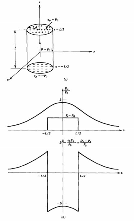
The solution for a single disk of surface charge was obtained in Section 2.3.5b. We superpose the results for the two disks taking care to shift the axial distance appropriately by \(\pm L/2\) yielding the concise solution for the displacement field:

\(D_{z} = \frac{P_{0}}{2} (\frac{(z + L/2)}{[a^{2} + (z + L/2)^{2}]^{1/2}} - \frac{(z-L/2)}{[a^{2} + (z-L/2)^{2}]^{1/2}})\)

The electric field is then

\(E_{z} = \left \{ \begin{matrix} D_{z}/\varepsilon_{0}, & \vert z \vert L/2 \\ (D_{z}-P_{0})/\varepsilon_{0} & \vert z \vert < L/2 \end{matrix} \right.\)

These results can be examined in various limits. If the radius a becomes very large, the electric field should approach that of two parallel sheets of surface charge \(\pm P_{0}\), as in Section 2.3.4b:

\(\lim_{a \rightarrow \infty} E_{z} = \left \{ \begin{matrix} 0, & \vert z \vert L/2 \\ -P_{0}/\varepsilon_{0}, & \vert z \vert < L/2 \end{matrix} \right.\)

with a zero displacement field everywhere.

In the opposite limit, for large z (z >> a, z >>L) far from the cylinder, the axial electric field dies off as the dipole field with \(\theta = 0\)

\(\lim_{z \rightarrow \infty} E_{z} = \frac{p}{2 \pi \varepsilon_{0}z^{3}}, \: \: \: p = P_{0} \pi a^{2}L\)

with effective dipole moment p given by the product of the total polarization charge at \(z = L/2, \: (P_{0} \pi a^{2})\), and the length L.

Normal Component of J

Applying the conservation of total current equation in Section 3.2.1 to the same Gaussian pillbox surface in Figure 3-12b results in contributions again only from the upper and lower surfaces labeled "a" and "b"

\[\textbf{n} \cdot (\textbf{J}_{2} - \textbf{J}_{1} + \frac{\partial}{\partial t} (\textbf{D}_{2} - \textbf{D}_{1}))=0 \]

where we assume that no surface currents flow along the interface. From (4), relating the surface charge density to the discontinuity in normal D, this boundary condition can also be written as

\[\textbf{n} \cdot (\textbf{J}_{2} - \textbf{J}_{1}) + \frac{\partial \sigma_{f}}{\partial t} = 0 \]

which tells us that if the current entering a surface is different from the current leaving, charge has accumulated at the interface. In the dc steady state the normal component of J is continuous across a boundary.