
3.10: Electrostatic Generators
- Page ID
- 54043
\( \newcommand{\vecs}[1]{\overset { \scriptstyle \rightharpoonup} {\mathbf{#1}} } \)
\( \newcommand{\vecd}[1]{\overset{-\!-\!\rightharpoonup}{\vphantom{a}\smash {#1}}} \)
\( \newcommand{\dsum}{\displaystyle\sum\limits} \)
\( \newcommand{\dint}{\displaystyle\int\limits} \)
\( \newcommand{\dlim}{\displaystyle\lim\limits} \)
\( \newcommand{\id}{\mathrm{id}}\) \( \newcommand{\Span}{\mathrm{span}}\)
( \newcommand{\kernel}{\mathrm{null}\,}\) \( \newcommand{\range}{\mathrm{range}\,}\)
\( \newcommand{\RealPart}{\mathrm{Re}}\) \( \newcommand{\ImaginaryPart}{\mathrm{Im}}\)
\( \newcommand{\Argument}{\mathrm{Arg}}\) \( \newcommand{\norm}[1]{\| #1 \|}\)
\( \newcommand{\inner}[2]{\langle #1, #2 \rangle}\)
\( \newcommand{\Span}{\mathrm{span}}\)
\( \newcommand{\id}{\mathrm{id}}\)
\( \newcommand{\Span}{\mathrm{span}}\)
\( \newcommand{\kernel}{\mathrm{null}\,}\)
\( \newcommand{\range}{\mathrm{range}\,}\)
\( \newcommand{\RealPart}{\mathrm{Re}}\)
\( \newcommand{\ImaginaryPart}{\mathrm{Im}}\)
\( \newcommand{\Argument}{\mathrm{Arg}}\)
\( \newcommand{\norm}[1]{\| #1 \|}\)
\( \newcommand{\inner}[2]{\langle #1, #2 \rangle}\)
\( \newcommand{\Span}{\mathrm{span}}\) \( \newcommand{\AA}{\unicode[.8,0]{x212B}}\)
\( \newcommand{\vectorA}[1]{\vec{#1}} % arrow\)
\( \newcommand{\vectorAt}[1]{\vec{\text{#1}}} % arrow\)
\( \newcommand{\vectorB}[1]{\overset { \scriptstyle \rightharpoonup} {\mathbf{#1}} } \)
\( \newcommand{\vectorC}[1]{\textbf{#1}} \)
\( \newcommand{\vectorD}[1]{\overrightarrow{#1}} \)
\( \newcommand{\vectorDt}[1]{\overrightarrow{\text{#1}}} \)
\( \newcommand{\vectE}[1]{\overset{-\!-\!\rightharpoonup}{\vphantom{a}\smash{\mathbf {#1}}}} \)
\( \newcommand{\vecs}[1]{\overset { \scriptstyle \rightharpoonup} {\mathbf{#1}} } \)
\(\newcommand{\longvect}{\overrightarrow}\)
\( \newcommand{\vecd}[1]{\overset{-\!-\!\rightharpoonup}{\vphantom{a}\smash {#1}}} \)
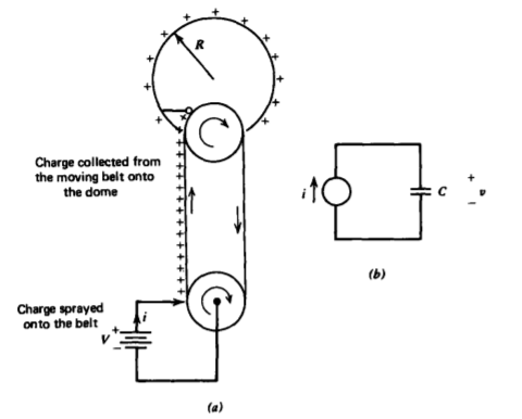
\(\newcommand{\avec}{\mathbf a}\) \(\newcommand{\bvec}{\mathbf b}\) \(\newcommand{\cvec}{\mathbf c}\) \(\newcommand{\dvec}{\mathbf d}\) \(\newcommand{\dtil}{\widetilde{\mathbf d}}\) \(\newcommand{\evec}{\mathbf e}\) \(\newcommand{\fvec}{\mathbf f}\) \(\newcommand{\nvec}{\mathbf n}\) \(\newcommand{\pvec}{\mathbf p}\) \(\newcommand{\qvec}{\mathbf q}\) \(\newcommand{\svec}{\mathbf s}\) \(\newcommand{\tvec}{\mathbf t}\) \(\newcommand{\uvec}{\mathbf u}\) \(\newcommand{\vvec}{\mathbf v}\) \(\newcommand{\wvec}{\mathbf w}\) \(\newcommand{\xvec}{\mathbf x}\) \(\newcommand{\yvec}{\mathbf y}\) \(\newcommand{\zvec}{\mathbf z}\) \(\newcommand{\rvec}{\mathbf r}\) \(\newcommand{\mvec}{\mathbf m}\) \(\newcommand{\zerovec}{\mathbf 0}\) \(\newcommand{\onevec}{\mathbf 1}\) \(\newcommand{\real}{\mathbb R}\) \(\newcommand{\twovec}[2]{\left[\begin{array}{r}#1 \\ #2 \end{array}\right]}\) \(\newcommand{\ctwovec}[2]{\left[\begin{array}{c}#1 \\ #2 \end{array}\right]}\) \(\newcommand{\threevec}[3]{\left[\begin{array}{r}#1 \\ #2 \\ #3 \end{array}\right]}\) \(\newcommand{\cthreevec}[3]{\left[\begin{array}{c}#1 \\ #2 \\ #3 \end{array}\right]}\) \(\newcommand{\fourvec}[4]{\left[\begin{array}{r}#1 \\ #2 \\ #3 \\ #4 \end{array}\right]}\) \(\newcommand{\cfourvec}[4]{\left[\begin{array}{c}#1 \\ #2 \\ #3 \\ #4 \end{array}\right]}\) \(\newcommand{\fivevec}[5]{\left[\begin{array}{r}#1 \\ #2 \\ #3 \\ #4 \\ #5 \\ \end{array}\right]}\) \(\newcommand{\cfivevec}[5]{\left[\begin{array}{c}#1 \\ #2 \\ #3 \\ #4 \\ #5 \\ \end{array}\right]}\) \(\newcommand{\mattwo}[4]{\left[\begin{array}{rr}#1 \amp #2 \\ #3 \amp #4 \\ \end{array}\right]}\) \(\newcommand{\laspan}[1]{\text{Span}\{#1\}}\) \(\newcommand{\bcal}{\cal B}\) \(\newcommand{\ccal}{\cal C}\) \(\newcommand{\scal}{\cal S}\) \(\newcommand{\wcal}{\cal W}\) \(\newcommand{\ecal}{\cal E}\) \(\newcommand{\coords}[2]{\left\{#1\right\}_{#2}}\) \(\newcommand{\gray}[1]{\color{gray}{#1}}\) \(\newcommand{\lgray}[1]{\color{lightgray}{#1}}\) \(\newcommand{\rank}{\operatorname{rank}}\) \(\newcommand{\row}{\text{Row}}\) \(\newcommand{\col}{\text{Col}}\) \(\renewcommand{\row}{\text{Row}}\) \(\newcommand{\nul}{\text{Nul}}\) \(\newcommand{\var}{\text{Var}}\) \(\newcommand{\corr}{\text{corr}}\) \(\newcommand{\len}[1]{\left|#1\right|}\) \(\newcommand{\bbar}{\overline{\bvec}}\) \(\newcommand{\bhat}{\widehat{\bvec}}\) \(\newcommand{\bperp}{\bvec^\perp}\) \(\newcommand{\xhat}{\widehat{\xvec}}\) \(\newcommand{\vhat}{\widehat{\vvec}}\) \(\newcommand{\uhat}{\widehat{\uvec}}\) \(\newcommand{\what}{\widehat{\wvec}}\) \(\newcommand{\Sighat}{\widehat{\Sigma}}\) \(\newcommand{\lt}{<}\) \(\newcommand{\gt}{>}\) \(\newcommand{\amp}{&}\) \(\definecolor{fillinmathshade}{gray}{0.9}\)3-10-1 Van de Graaff Generator
In the 1930s, reliable means of generating high voltages were necessary to accelerate charged particles in atomic studies. In 1931, Van de Graaff developed an electrostatic generator where charge is sprayed onto an insulating moving belt that transports this charge onto a conducting dome, as illustrated in Figure 3-37a. If the dome was considered an isolated sphere of radius R, the capacitance is given as \(C= 4 \pi \varepsilon_{0}R\). The transported charge acts as a current source feeding this capacitance, as in Figure 3-37b, so that the dome voltage builds up linearly with time:
\[i = C \frac{dv}{dt} \Rightarrow v = \frac{i}{C}t \]
This voltage increases until the breakdown strength of the surrounding atmosphere is reached, whereupon a spark discharge occurs. In air, the electric field breakdown strength Eb is 3 x 10⁶ V/m. The field near the dome varies as \(E_{r} = VR/r^{2}\) which is maximum at r= R, which implies a maximum voltage of Vmax= EbR. For Vmax = 106 V, the radius of the sphere
must be \(R \approx \frac{1}{3}\) mi so that the capacitance is \(C \approx 37\) pf. With a charging current of one microampere, it takes \(t \approx 37\) sec to reach this maximum voltage.
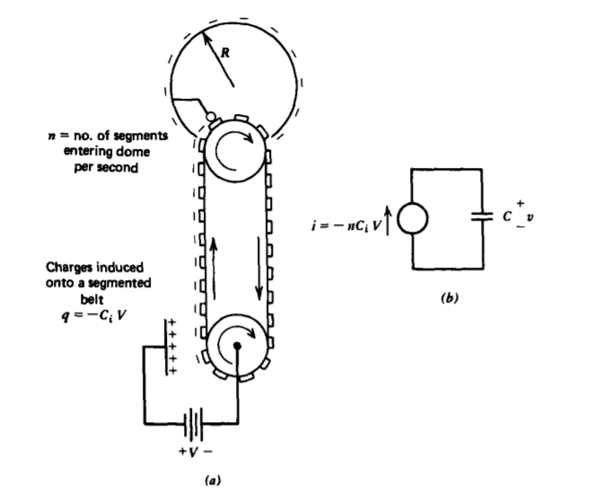
3-10-2 Self-Excited Electrostatic Induction Machines
In the Van de Graaff generator, an external voltage source is necessary to deposit charge on the belt. In the late 1700s, self-excited electrostatic induction machines were developed that did not require any external electrical source. To understand how these devices work, we modify the Van de Graaff generator configuration, as in Figure 3-38a, by putting conducting segments on the insulating belt. Rather than spraying charge, we place an electrode at voltage V with respect to the lower conducting pulley so that opposite polarity charge is induced on the moving segments. As the segments move off the pulley, they carry their charge with them. So far, this device is similar to the Van de Graaff generator using induced charge rather than sprayed charge and is described by the same equivalent circuit where the current source now depends on the capacitance Ci between the inducing electrode and the segmented electrodes, as in Figure 3-38b.
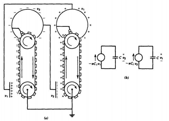
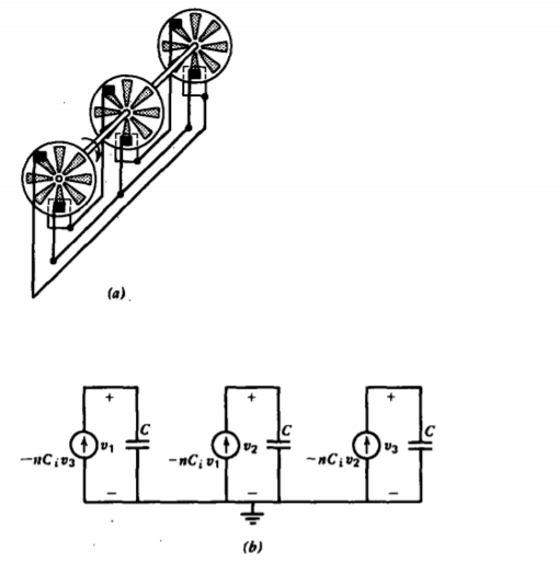
Now the early researchers cleverly placed another induction machine nearby as in Figure 3-39a. Rather than applying a voltage source, because one had not been invented yet, they electrically connected the dome of each machine to the inducer electrode of the other. The induced charge on one machine was proportional to the voltage on the other dome. Although no voltage is applied, any charge imbalance on an inducer electrode due to random noise or stray charge will induce an opposite charge on the moving segmented belt that carries this charge to the dome of which some appears on the other inducer electrode where the process is repeated with opposite polarity charge. The net effect is that the charge on the original inducer has been increased.
More quantitatively, we use the pair of equivalent circuits in Figure 3-39b to obtain the coupled equations
\[-nC_{i}v_{1} = C \frac{dv_{2}}{dt}, \: \: \: \: -nC_{i}v_{2} = C \frac{dv_{1}}{dt} \]
where n is the number of segments per second passing through the dome. All voltages are referenced to the lower pulleys that are electrically connected together. Because these
are linear constant coefficient differential equations, the solutions must be exponentials:
\[v_{1} = \hat{\textrm{V}}_{1}e^{st}, \: \: \: \: v_{2} = \hat{\textrm{V}}_{2}e^{st} \]
Substituting these assumed solutions into (2) yields the following characteristic roots:
\[s^{2} = \bigg(\frac{nC_{i}}{C}\bigg)^{2} \Rightarrow s = \pm \frac{nC_{i}}{C} \]
so that the general solution is
\[v_{1} = A_{1}e^{(nC_{i}/C)t} + A_{2}e^{-(nC_{i}/C)t} \\ v_{2}= -A_{1}e^{(nC_{i}/C)t} + A_{2}e^{-(nC_{i}/C)t} \]
where A1 and A2 are determined from initial conditions.
The negative root of (4) represents the uninteresting decaying solutions while the positive root has solutions that grow unbounded with time. This is why the machine is self-excited. Any initial voltage perturbation, no matter how small, increases without bound until electrical breakdown is reached. Using representative values of n = 10, Ci= 2 pf, and C= 10 pf, we have that \(s = \pm 2\) so that the time constant for voltage build-up is about one-half second.
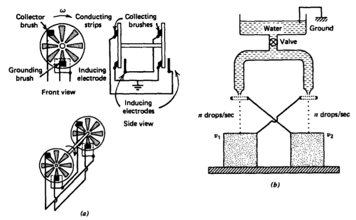
The early electrical scientists did not use a segmented belt but rather conducting disks embedded in an insulating wheel that could be turned by hand, as shown for the Wimshurst machine in Figure 3-40a. They used the exponentially growing voltage to charge up a capacitor called a Leyden jar (credited to scientists from Leyden, Holland), which was a glass bottle silvered on the inside and outside to form two electrodes with the glass as the dielectric.
An analogous water drop dynamo was invented by Lord Kelvin (then Sir W. Thomson) in 1861, which replaced the rotating disks by falling water drops, as in Figure 3-40b. All these devices are described by the coupled equivalent circuits in Figure 3-39b.
3-10-3 Self-Excited Three-Phase Alternating Voltages
In 1967, Euerle* modified Kelvin's original dynamo by adding a third stream of water droplets so that three-phase alternating voltages were generated. The analogous three phase Wimshurst machine is drawn in Figure 3-41a with equivalent circuits in Figure 3-41b. Proceeding as we did in (2) and (3),
\[\begin{matrix} -nC_{i}v_{1}=C\frac{dv_{2}}{dt}, & v_{1} = \hat{\textrm{V}}_{1}e^{st} \\ -nC_{i}v_{2}=C \frac{dv_{3}}{dt}, & v_{2}= \hat{\textrm{V}}_{2}e^{st} \\ -nC_{i}v_{3}=C \frac{dv_{1}}{dt}, & v_{3} = \hat{\textrm{V}}_{3}e^{st} \end{matrix} \]
equation (6) can be rewritten as
\[ \left[ \begin{matrix} nC_{i} & C_{s} & 0 \\ 0 & nC_{i} & C_{s} \\ C_{s} & 0 & nC_{i} \end{matrix} \right] \left[ \begin{matrix} \hat{\textrm{V}}_{1} \\ \hat{\textrm{V}}_{2} \\ \hat{\textrm{V}}_{3} \end{matrix} \right] = 0 \]
which requires that the determinant of the coefficients of \(\hat{\textrm{V}}_{1}\), \(\hat{\textrm{V}}_{2}\), and \(\hat{\textrm{V}}_{3}\) be zero:
\[(nC_{i})^{3} + (cs)^{3} = 0 \Rightarrow s = \bigg(\frac{nC_{i}}{C} \bigg)^{1/3} (-1)^{1/3} \\ = \bigg(\frac{nC_{i}}{C} \bigg)^{1/3} e^{j(\pi/3)(2r-1)}, \: \: \: r = 1, 2, 3 \\ \Rightarrow s_{1} = - \frac{nC_{i}}{C} \\ s_{2,3} = \frac{nC_{i}}{2C}[1 \pm \sqrt{3}j] \]
where we realized that (- 1)1/3 has three roots in the complex plane. The first root is an exponentially decaying solution, but the other two are complex conjugates where the positive real part means exponential growth with time while the imaginary part gives the frequency of oscillation. We have a self-excited three-phase generator as each voltage for the unstable modes is 120° apart in phase from the others:
\[\frac{\hat{\textrm{V}}_{2}}{\hat{\textrm{V}}_{1}} = \frac{\hat{\textrm{V}}_{3}}{\hat{\textrm{V}}_{2}}={\hat{\textrm{V}}_{1}}{\hat{\textrm{V}}_{3}} = - \frac{nC_{i}}{Cs_{2,3}} = -\frac{1}{2}(1 \pm \sqrt{3}j) = e^{\pm j(2/3) \pi} \]
Using our earlier typical values following (5), we see that the oscillation frequencies are very low, \(f = (1/2 \pi)\) Im(s) \(\approx\) 0.28 Hz.
* W C. Euerle, "A Novel Method of Generating Polyphase Power," M.S. Thesis, Massachusetts Institute of Technology, 1967. See also J. R. Melcher, Electric Fields and Moving Media, IEEE Trans. Education E-17 (1974), pp. 100-110, and the film by the same title produced for the National Committee on Electrical Engineering Films by the Educational Development Center, 39 Chapel St., Newton, Mass. 02160.
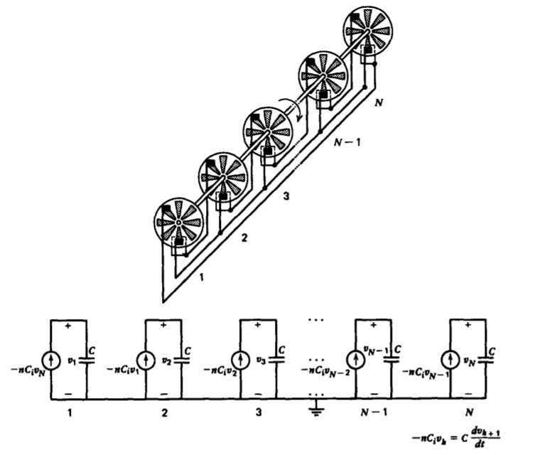
3-10-4 Self-Excited Multi-frequency Generators
If we have N such generators, as in Figure 3-42, with the last one connected to the first one, the kth equivalent circuit yields
\[-nC_{i} \hat{\textrm{V}}_{k} = Cs \hat{\textrm{V}}_{k + 1} \]
This is a linear constant coefficient difference equation. Analogously to the exponential time solutions in (3) valid for linear constant coefficient differential equations, solutions to (10) are of the form
\[\textrm{V}_{k} = A \lambda^{k} \]
where the characteristic root \(\lambda\) is found by substitution back into (10) to yield
\[-nC_{i}A \lambda^{k} = CsA \lambda^{k+1} \Rightarrow \lambda = - nC_{i}/Cs \]
Since the last generator is coupled to the first one, we must have that
\[\textrm{V}_{N+1} = V_{1} \Rightarrow \lambda^{N+1} = \lambda^{1} \\ \Rightarrow \lambda^{N} = 1 \\ \lambda = 1^{1/N} = e^{j 2 wr/N}, \: \: \: \: \: r = 1,2,3,...,N \]
where we realize that unity has N complex roots.
The system natural frequencies are then obtained from (12) and (13) as
\[s = - \frac{nC_{i}}{C \lambda} = - \frac{nC_{i}}{C} e^{-j2 \pi r/N}, \: \: \: \: r=1,2,...,N \]
We see that for N =2 and N= 3 we recover the results of (4) and (8). All the roots with a positive real part of s are unstable and the voltages spontaneously build up in time with oscillation frequencies \(\omega_{0}\) given by the imaginary part of s.
\[\omega_{0} = \vert \textrm{Im} (s) \vert = \frac{nC_{i}}{C} \vert \sin 2 \pi r/N \vert \]