3.9: Fields and their Forces

3-9-1 Force Per Unit Area on a Sheet of Surface Charge

A confusion arises in applying Coulomb's law to find the perpendicular force on a sheet of surface charge as the normal electric field is different on each side of the sheet. Using the over-simplified argument that half the surface charge resides on each side of the sheet yields the correct force

\[\textbf{F} = \frac{1}{2} \int_{S} \sigma_{f} (\textbf{E}_{1} + \textbf{E}_{2}) d \textrm{S} \]

where, as shown in Figure 3-33a, E₁ and E₂ are the electric fields on each side of the sheet. Thus, the correct field to use is the average electric field \(\frac{1}{2}(\textbf{E}_{1} + \textbf{E}_{2})\) across the sheet.

For the tangential force, the tangential components of E are continuous across the sheet (\(E_{1t} = E_{2t} \approx E_{t}\)) so that

\[f_{t} = \frac{1}{2} \int_{S} \sigma_{f}(E_{1t} + E_{2t}) d \textrm{S} = \int_{S} \sigma_{f}E_{t} d \textrm{S} \]

Figure 3-33 (a) The normal component of electric field is discontinuous across the sheet of surface charge. (b) The sheet of surface charge can be modeled as a thin layer of volume charge. The electric field then varies linearly across the volume.

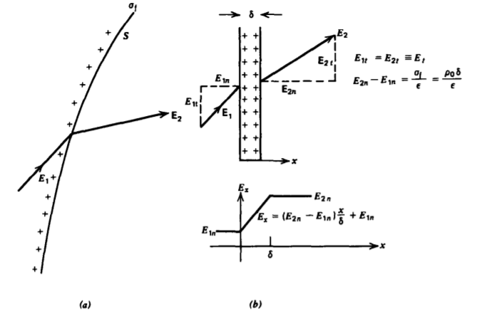
The normal fields are discontinuous across the sheet so that the perpendicular force is

\[\sigma_{f} = \varepsilon (E_{2n} - E_{1n}) \Rightarrow f_{n} = \frac{1}{2} \int_{S} \varepsilon (E_{2n}-E_{1n})(E_{1n} + E_{2n}) d \textrm{S} \\ = \frac{1}{2} \int_{S} \varepsilon (E_{2n}^{2} - E_{1n}^{2})d \textrm{S} \]

To be mathematically rigorous we can examine the field transition through the sheet more closely by assuming the surface charge is really a uniform volume charge distribution \(\rho_{0}\) of very narrow thickness \(\delta\), as shown in Figure 3-33b. Over the small surface element dS, the surface appears straight so that the electric field due to the volume charge can then only vary with the coordinate x perpendicular to the surface. Then the point form of Gauss's law within the volume yields

\[\frac{dE_{x}}{dx} = \frac{\rho_{0}}{\varepsilon} \Rightarrow E_{x} = \frac{\rho_{0}x}{\varepsilon} + \textrm{const} \]

The constant in (4) is evaluated by the boundary conditions on the normal components of electric field on each side of the sheet

\[E_{x}(x=0) = E_{1n}, \: \: \: \: \: E_{x}(x = \delta) = E_{2n} \]

so that the electric field is

\[E_{x} = (E_{2n} - E_{1n}) \frac{x}{\delta} + E_{1n} \]

As the slab thickness \(\delta\) becomes very small, we approach a sheet charge relating the surface charge density to the discontinuity in electric fields as

\[\lim_{\rho_{0} \rightarrow \infty \\ \delta \rightarrow 0} \rho_{0} \delta = \sigma_{f} = \varepsilon (E_{2n} - E_{1n}) \]

Similarly the force per unit area on the slab of volume charge is

\[F_{x} = \int_{0}^{|delta} \rho_{0}E_{x}dx \\ = \int_{0}^{\delta} \rho_{0} \bigg[ (E_{2n} - E_{1n}) \frac{x}{\delta} + E_{1n} \bigg] dx \\ = \bigg[ \rho_{0} (E_{2n} - E_{1n}) \frac{x^{2}}{2 \delta} + E_{1n}x \bigg] \bigg|_{0}^{\delta} \\ = \frac{\rho_{0} \delta}{2} (E_{1n} + E_{2n}) \]

In the limit of (7), the force per unit area on the sheet of surface charge agrees with (3):

\[\lim_{\rho_{0} \delta = \sigma_{f}} F_{x} = \frac{\sigma_{f}}{2}(E_{1n} + E_{2n}) = \frac{\varepsilon}{2} (E_{2n}^{2} -E_{1n}^{2}) \]

3-9-2 Forces on a Polarized Medium

(a) Force Density

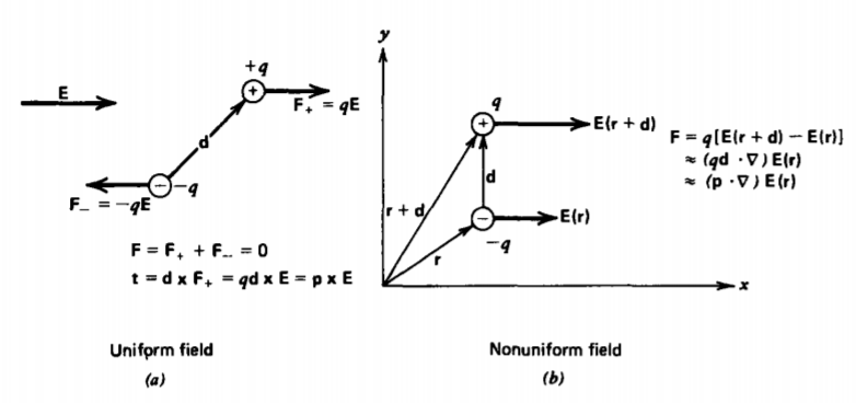
In a uniform electric field there is no force on a dipole because the force on each charge is equal in magnitude but opposite in direction, as in Figure 3-34a. However, if the dipole moment is not aligned with the field there is an aligning torque given by t = p x E. The torque per unit volume T on a polarized medium with N dipoles per unit volume is then

\[\textbf{T} = N \textbf{t} = N \textbf{p} \times \textbf{P} \times \textbf{E} \]

Figure 3-34 (a) A torque is felt by a dipole if its moment is not aligned with the electric field. In a uniform electric field there is no net force on a dipole because the force on each charge is equal in magnitude but opposite in direction. (b) There is a net force on a dipole only in a nonuniform field.

For a linear dielectric, this torque is zero because the polarization is induced by the field so that P and E are in the same direction.

A net force can be applied to a dipole if the electric field is different on each end, as in Figure 3-34b:

\[\textbf{f} = -q[\textbf{E}(\textbf{r}) - \textbf{E}(\textbf{r} + \textbf{d})] \]

For point dipoles, the dipole spacing d is very small so that the electric field at r + d can be expanded in a Taylor series as

\[\textbf{E}(\textbf{E} + \textbf{d}) \approx \textbf{E} (\textbf{r}) + d_{x} \frac{\partial}{\partial x} \textbf{E} (\textbf{r}) + d_{y} \frac{\partial}{\partial y} \textbf{E}(\textbf{r}) + d_{z} \frac{\partial}{\partial z} \textbf{E}(\textbf{r}) = \textbf{E}(\textbf{r}) + (\textbf{d} \cdot \nabla) \textbf{E}(\textbf{r}) \]

Then the force on a point dipole is

\[\textbf{f} = (q \textbf{d} \cdot \nabla) \textbf{E}(\textbf{r}) = (\textbf{p} \cdot \nabla) \textbf{E}(\textbf{r}) \]

If we have a distribution of such dipoles with number density N, the polarization force density is

\[\textbf{F} + N \textbf{f} = (N \textbf{p} \cdot \nabla) \textbf{E} = (\textbf{P} \cdot \nabla) \textbf{E} \]

Of course, if there is any free charge present we must also add the coulombic force density \(\rho_{f} \textbf{E}\).

(b) Permanently Polarized Medium

A permanently polarized material with polarization \(P_{0}\textbf{i}\), is free to slide between parallel plate electrodes, as is shown in Figure 3-35.

Figure 3-35 (a) A permanently polarized electret partially inserted into a capacitor has a force on it due to the Coulombic attraction between the dipole charges and the surface charge on the electrodes. The net force arises in the fringing field region as the end of the dipole further from the electrode edge feels a smaller electric field. Depending on the voltage magnitude and polarity, the electret can be pulled in or pushed out of the capacitor. (b) A linear dielectric is always attracted into a free space capacitor because of the net force on dipoles in the nonuniform field. The dipoles are now aligned with the electric field, no matter the voltage polarity

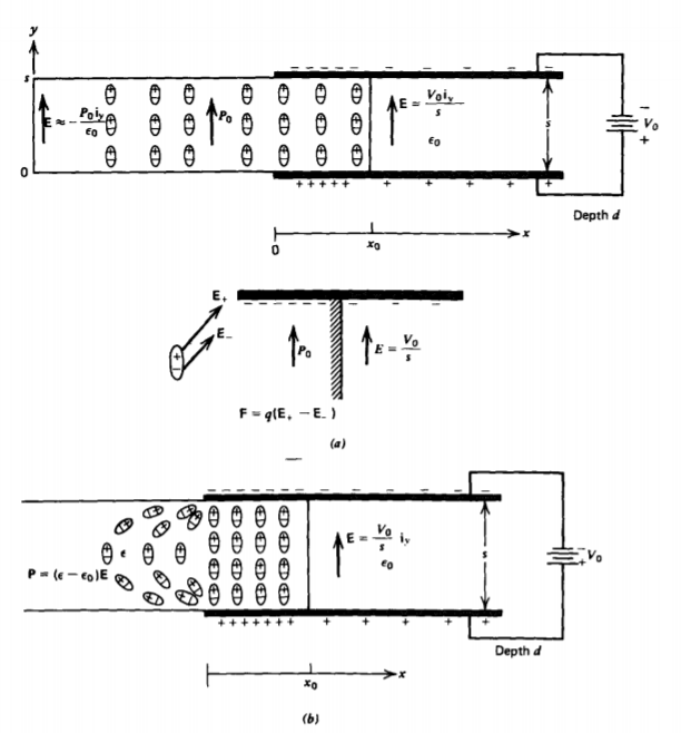
We only know the electric field in the interelectrode region and from Example 3-2 far away from the electrodes:

\[E_{y} (x = x_{0}) = \frac{V_{0}}{s}, \: \: \: E_{y}(x = - \infty) = - \frac{P_{0}}{\varepsilon_{0}} \]

Unfortunately, neither of these regions contribute to the force because the electric field is uniform and (14) requires a field gradient for a force. The force arises in the fringing fields near the electrode edges where the field is nonuniform and, thus, exerts less of a force on the dipole end further from the electrode edges. At first glance it looks like we have a difficult problem because we do not know the fields where the force acts. However, because the electric field has zero curl,

\[\nabla \times \textbf{E} = 0 \Rightarrow \frac{\partial E_{x}}{\partial y} = \frac{\partial E_{y}}{\partial x} \]

the x component of the force density can be written as

\[F_{x} =P_{y} \frac{\partial E_{x}}{\partial y} \\ = P_{y} \frac{\partial E_{y}}{\partial x} \\ = \frac{\partial}{\partial x} (P_{y}E_{y})-E_{y} \frac{\partial P_{y}}{\partial x} \nearrow^{0} \]

The last term in (17) is zero because \(P_{y} =P_{0}\) is a constant. The total x directed force is then

\[f_{x} = \int F_{x} dx dy dz \\ = \int_{x = i \infty}^{x_{0}} \int_{y=0}^{s} \int_{z = 0}^{d} \frac{\partial}{\partial x} (P_{y}E_{y}) dx dy dz \]

We do the x integration first so that the y and z integrations are simple multiplications as the fields at the limits of the x integration are independent of y and z:

\[f_{x} = P_{0}E_{y}sd \|_{x= - \infty}^{x_{0}} = P_{0}V_{0}d + \frac{P_{0}^{2}sd}{\varepsilon_{0}} \]

There is a force pulling the electret between the electrodes even if the voltage were zero due to the field generated by the surface charge on the electrodes induced by the electret. This force is increased if the imposed electric field and polarization are in the same direction. If the voltage polarity is reversed, the force is negative and the electret is pushed out if the magnitude of the voltage exceeds \(P_{0}s/\varepsilon_{0}\).

(c) Linearly Polarized Medium

The problem is different if the slab is polarized by the electric field, as the polarization will then be in the direction of the electric field and thus have x and y components in the fringing fields near the electrode edges where the force arises, as in Figure 3-35b. The dipoles tend to line up as shown with the positive ends attracted towards the negative electrode and the negative dipole ends towards the positive electrode. Because the farther ends of the dipoles are in a slightly weaker field, there is a net force to the right tending to draw the dielectric into the capacitor.

The force density of (14) is

\[F_{x} = P_{x} \frac{\partial E_{x}}{\partial x} + P_{y} \frac{\partial E_{x}}{\partial y} = (\varepsilon - \varepsilon_{0}) \bigg( E_{x} \frac{\partial E_{x}}{\partial x} + E_{y} \frac{\partial E_{x}}{\partial y} \bigg) \]

Because the electric field is curl free, as given in (16), the force density is further simplified to

\[F_{x} = \frac{(\varepsilon- \varepsilon_{0})}{2} \frac{\partial}{\partial x}(E_{x}^{2} + E_{y}^{2}) \]

The total force is obtained by integrating (21) over the volume of the dielectric:

\[f_{x} = \int_{X = - \infty}^{x_{0}} \int_{y=0}^{s} \int_{z=0}^{d} \frac{(\varepsilon - \varepsilon_{0})}{2} \frac{\partial}{\partial x} (E_{x}^{2} + E_{y}^{2}) dx dy dz \\ = \frac{(\varepsilon - \varepsilon_{0})sd}{2} (E_{x}^{2} + E_{y}^{2}) \|_{x = - \infty}^{x_{0}} = \frac{(\varepsilon - \varepsilon_{0})}{2} \frac{V_{0}^{2}d}{s} \]

where we knew that the fields were zero at \(x = - \infty\) and uniform at \(x = x_{0}\):

\[E_{y}(x_{0}) = V_{0}/s, \: \: \: E_{x}(x_{0}) = 0 \]

The force is now independent of voltage polarity and always acts in the direction to pull the dielectric into the capacitor if \(\varepsilon > \varepsilon_{0}\)

3-9-3 Forces on a Capacitor

Consider a capacitor that has one part that can move in the x direction so that the capacitance depends on the coordinate x:

\[q = C(x)v \]

The current is obtained by differentiating the charge with respect to time:

\[i = \frac{dq}{dt} = \frac{d}{dt} [C(x)v] = C(x) \frac{dv}{dt} + v \frac{dC(x)}{dt} = C(x) \frac{dv}{dt} + v \frac{dC(x)}{dx} \frac{dx}{dt} \]

Note that this relation has an extra term over the usual circuit formula, proportional to the speed of the moveable member, where we expanded the time derivative of the capacitance by the chain rule of differentiation. Of course, if the geometry is fixed and does not change with time (dx/dt = 0), then (25) reduces to the usual circuit expression. The last term is due to the electro-mechanical coupling.

The power delivered to a time-dependent capacitance is

\[p = v \textbf{i} = v \frac{d}{dt}[C(x)v] \]

which can be expanded to the form

\[p = \frac{d}{dt}[\frac{1}{2} C(x)v^{2}] + \frac{1}{2}v^{2}\frac{dC(x)}{dt} \\ = \frac{d}{dt} [\frac{1}{2} C (x)v^{2}] + \frac{1}{2} v^{2} \frac{dC(x)}{dx} \frac{dx}{dt} \]

where the last term is again obtained using the chain rule of differentiation. This expression can be put in the form

\[p = \frac{dW}{dt} + f_{x}\frac{dx}{dt} \]

where we identify the power p delivered to the capacitor as going into increasing the energy storage W and mechanical power \(f_{x} dx/dt\) in moving a part of the capacitor:

\[W = \frac{1}{2} C(x) v^{2}, \: \: \: \: f_{x} = \frac{1}{2} v^{2} \frac{dC(x)}{dx} \]

Using (24), the stored energy and force can also be expressed in terms of the charge as

\[W = \frac{1}{2} \frac{q^{2}}{C(x)}, \: \: \: f_{x} = \frac{1}{2} \frac{q^{2}}{C^{2}(x)} \frac{dC(x)}{dx} = - \frac{1}{2}q^{2} \frac{d[1/C(x)]}{dx} \]

To illustrate the ease in using (29) or (30) to find the force, consider again the partially inserted dielectric in Figure 3-35b. The capacitance when the dielectric extends a distance x into the electrodes is

\[C(x) = \frac{\varepsilon x d}{s} + \varepsilon_{0}\frac{(l-x)d}{s} \]

so that the force on the dielectric given by (29) agrees with (22):

\[f_{x} = \frac{1}{2} V_{0}^{2} \frac{dC(x)}{dx} = \frac{1}{2}(\varepsilon - \varepsilon_{0}) \frac{V_{0}^{2}d}{s} \]

Note that we neglected the fringing field contributions to the capacitance in (31) even though they are the physical origin of the force. The results agree because this extra capacitance does not depend on the position x of the dielectric when x is far from the electrode edges.

This method can only be used for linear dielectric systems described by (24). It is not valid for the electret problem treated in Section 3-9-2b because the electrode charge is not linearly related to the voltage, being in part induced by the electret.

EXAMPLE 3-4: FORCE ON A PARALLEL PLATE CAPACITOR

Two parallel, perfectly conducting electrodes of area A and a distance x apart are shown in Figure 3-36. For each of the following two configurations, find the force on the upper electrode in the x direction when the system is constrained to constant voltage V_o or constant charge Q_o.

Figure 3-36 A parallel plate capacitor (a) immersed within a dielectric fluid or with (b) a free space region in series with a solid dielectric.

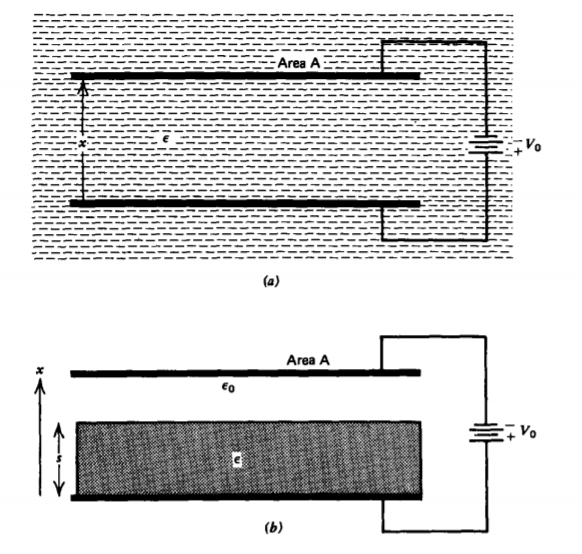
(a) Liquid Dielectric

The electrodes are immersed within a liquid dielectric with permittivity \(\varepsilon\), as shown in Figure 3-36a.

(b) Solid Dielectric

A solid dielectric with permittivity e of thickness s is inserted between the electrodes with the remainder of space having permittivity eo, as shown in Figure 3-36b.

Answer

a) The capacitance of the system is

\(C(x) = \varepislon A/x\)

so that the force from (29) for constant voltage is

\(f_{x} = \frac{1}{2} V_{0}^{2} \frac{dC(x)}{dx} = - \frac{1}{2} \frac{\varepsilon A V_{0}^{2}}{x^{2}}\)

The force being negative means that it is in the direction opposite to increasing x, in this case downward. The capacitor plates attract each other because they are oppositely charged and opposite charges attract. The force is independent of voltage polarity and gets infinitely large as the plate spacing approaches zero. The result is also valid for free space with \(\varepsilon = \varepsilon_{0}\). The presence of the dielectric increases the attractive force.

If the electrodes are constrained to a constant charge Q_o the force is then attractive but independent of x:

\(f_{x} = - \frac{1}{2} Q_{0}^{2} \frac{d}{dx} \frac{1}{C(x)}= - \frac{1}{2} \frac{Q_{0}^{2}}{\varepsilon A}\)

For both these cases, the numerical value of the force is the same because Qo and Vo are related by the capacitance, but the functional dependence on x is different. The presence of a dielectric now decreases the force over that of free space.

(b) Solid Dielectric

A solid dielectric with permittivity \(\varepsilon\) of thickness s is inserted between the electrodes with the remainder of space having permittivity \(\varepsilon\), as shown in Figure 3-36b.

The total capacitance for this configuration is given by the series combination of capacitance due to the dielectric block and the free space region:

\[C(x) = \frac{\varepsilon \varepsilon_{0}A}{\varepsilon_{0}s + \varepsilon (x-s)} \]

The force on the upper electrode for constant voltage is

\[f_{x} = \frac{1}{2} V_{0}^{2} \frac{d}{dx} C(x) = - \frac{\varepsilon^{2} \varepsilon_{0}A V_0^{2}}{2 [\varepsilon_{0}s + \varepsilon(x-s)]^{2}} \]

If the electrode just rests on the dielectric so that x = s, the force is

\[f_{x}= - \frac{\varepsilon^{2}AV_{0}^{2}}{2 \varepsilon_{0}s^{2}}. \]

This result differs from that of part (a) when x = s by the factor \(\varepsilon_{r}= \varepsilon/\varepsilon_{0}\) because in this case moving the electrode even slightly off the dielectric leaves a free space region in between. In part (a) no free space gap develops as the liquid dielectric fills in the region, so that the dielectric is always in contact with the electrode. The total force on the electrode-dielectric interface is due to both free and polarization charge

With the electrodes constrained to constant charge, the force on the upper electrode is independent of position and also independent of the permittivity of the dielectric block:

\[f_{x} = - \frac{1}{2}Q_{0}^{2} \frac{d}{dx} \frac{1}{C(x)} = - \frac{1}{2} \frac{Q_{0}^{2}}{\varepsilon_{0}A} \]