3.8: Energy Stored in a Dielectric Medium

The work needed to assemble a charge distribution is stored as potential energy in the electric field because if the charges are allowed to move this work can be regained as kinetic energy or mechanical work.

3-8-1 Work Necessary to Assemble a Distribution of Point Charges

(a) Assembling the Charges

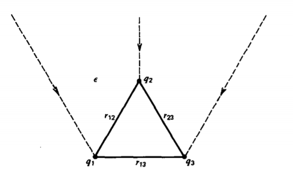
Let us compute the work necessary to bring three already existing free charges q₁, q₂, and q₃ from infinity to any position, as in Figure 3-28. It takes no work to bring in the first charge as there is no electric field present. The work necessary to bring in the second charge must overcome the field due to the first charge, while the work needed to bring in the third charge must overcome the fields due to both other charges. Since the electric potential developed in Section 2-5-3 is defined as the work per unit charge necessary to bring a point charge in from infinity, the total work necessary to bring in the three charges is

\[ W=q_1(0)+q_2\left(\frac{q_1}{4 \pi \varepsilon r_{12}}\right)+q_3\left(\frac{q_1}{4 \pi \varepsilon r_{13}}+\frac{q_2}{4 \pi \varepsilon r_{23}}\right) \]

where the final distances between the charges are defined in Figure 3-28 and we use the permittivity \(\varepsilon\) of the medium. We can rewrite (1) in the more convenient form

\[W = \frac{1}{2} \left \{ \begin{matrix} q_{1} \bigg[ \frac{q_{2}}{4 \pi \varepsilon r_{12}} + \frac{q_{3}}{4 \pi \varepsilon r_{13}} \bigg] + q_{2} \bigg[\frac{q_{1}}{4 \pi \varepsilon r_{12}} + \frac{q_{3}}{4 \pi \varepsilon r_{23}} \bigg] + q-{3} \bigg[\frac{q_{1}}{4 \pi \varepsilon r_{13}} + \frac{q_{2}}{4 \pi \varepsilon r_{23}} \bigg] \end{matrix} \right \} \]

Figure 3-28 Three already existing point charges are brought in from an infinite distance to their final positions.

where we recognize that each bracketed term is just the potential at the final position of each charge and includes contributions from all the other charges, except the one located at the position where the potential is being evaluated:

\[W = \frac{1}{2} [q_{1} V_{1} + q_{2}V_{2} + q_{3}V_{3} \]

Extending this result for any number N of already existing free point charges yield

\[W = \frac{1}{2} \sum_{n=1}^{N} q_{n}V_{n} \]

The factor of \(\frac{1}{2}\) arises because the potential of a point charge at the time it is brought in from infinity is less than the final potential when all the charges are assembled.

(b) Binding Energy of a Crystal

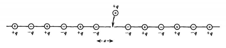
One major application of (4) is in computing the largest contribution to the binding energy of ionic crystals, such as salt (NaCI), which is known as the Madelung electrostatic energy. We take a simple one-dimensional model of a crystal consisting of an infinitely long string of alternating polarity point charges \(\pm q\) a distance a apart, as in Figure 3-29. The average work necessary to bring a positive charge as shown in Figure 3-29 from infinity to its position on the line is obtained from (4) as

\[W = \frac{1}{2} \frac{2q^{2}}{4 \pi \varepsilon a} \bigg[ -1 + \frac{1}{2} - \frac{1}{3} + \frac{1}{4} - \frac{1}{5} + \frac{1}{6} - ... \bigg] \]

The extra factor of 2 in the numerator is necessary because the string extends to infinity on each side. The infinite series is recognized as the Taylor series expansion of the logarithm

\[\ln(1 + x) = x - \frac{x^{2}}{2} + \frac{x^{3}}{3} - \frac{x^{4}}{4} + \frac{x^{5}}{5} - ... \]

Figure 3-29 A one-dimensional crystal with alternating polarity charges \(\pm q\) a distance a apart

where x = 1 so that*

\[W = \frac{-q^{2}}{4 \pi \varepsilon a} \ln 2 \]

This work is negative because the crystal pulls on the charge as it is brought in from infinity. This means that it would take positive work to remove the charge as it is bound to the crystal. A typical ion spacing is about 3 \(\AA\) (3 x 10^-10 m) so that if q is a single proton (q= 1.6x 10^-19 coul), the binding energy is \(W \approx 5.3 \times 10^{-19}\) joule. Since this number is so small it is usually more convenient to work with units of energy per unit electronic charge called electron volts (ev), which are obtained by dividing W by the charge on an electron so that, in this case, \(W \approx 3.3\) ev.

If the crystal was placed in a medium with higher permittivity, we see from (7) that the binding energy decreases. This is why many crystals are soluble in water, which has a relative dielectric constant of about 80.

3-8-2 Work Necessary to Form a Continuous Charge Distribution

Not included in (4) is the self-energy of each charge itself or, equivalently, the work necessary to assemble each point charge. Since the potential V from a point charge q is proportional to q, the self-energy is proportional q². However, evaluating the self-energy of a point charge is difficult because the potential is infinite at the point charge.

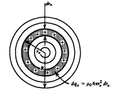
To understand the self-energy concept better it helps to model a point charge as a small uniformly charged spherical volume of radius R with total charge \(Q = \frac{4}{3} \pi R^{3} \rho_{0}\). We assemble the sphere of charge from spherical shells, as shown in Figure 3-30, each of thickness dr_n and incremental charge \(dq_{n} = 4 \pi r_{n}^{2}dr_{n}\rho_{0}\). As we bring in the nth shell to be placed at radius r_n the total charge already present and the potential there are

\[q_{n} = \frac{4}{3} \pi r_{n}^{3}\rho_{0}, \: \: \: V_{n} = \frac{q_{n}}{4 \pi \varepsilon r_{n}} = \frac{r_{n}^{2}\rho_{0}}{3 \varepsilon} \]

Figure 3-30 A point charge is modelled as a small uniformly charged sphere. It is assembled by bringing in spherical shells of differential sized surface charge elements from infinity.

so that the work required to bring in the nth shell is

\[dW_{n} = V_{n} dq_{n} = \frac{\rho_{0}^{2}4 \pi r_{n}^{4}}{3 \varepsilon} dr_{n} \]

The total work necessary to assemble the sphere is obtained by adding the work needed for each shell:

\[W = \int dW_{n} = \int_{0}^{R} \frac{4 \pi \rho_{0}^{2}r^{4}}{3 \varepsilon} dr = \frac{4 \pi \rho_{0}^{2} R^{5}}{15 \varepsilon} = \frac{3Q^{2}}{20 \pi \varepsilon R} \]

For a finite charge Q of zero radius the work becomes infinite. However, Einstein's theory of relativity tells us that this work necessary to assemble the charge is stored as energy that is related to the mass as

\[W = mc^{2} = \frac{3Q^{2}}{20 \pi \varepsilon R} \Rightarrow R = \frac{3Q^{2}}{20 \pi \varepsilon mc^{2}} \]

which then determines the radius of the charge. For the case of an electron (Q = 1.6 x 10^-19 coul, m = 9.1 x 10^-31 kg) in free space (\(\varepsilon = \varepsilon_{0}\)= 8.854 x 10^-12 farad/m), this radius is

\[R_{\textrm{electron}} = \frac{3(1.6 \times 10^{-19})^{2}}{20 \pi (8.854 \times 10^{-12})(9.1 \times 10^{-31})(3 \times 10^{8})^{2}} \approx 1.69 \times 10^{-15} \textrm{m} \]

We can also obtain the result of (10) by using (4) where each charge becomes a differential element dq, so that the summation becomes an integration over the continuous free charge distribution:

\[W = \frac{1}{2} \int_{\textrm{all } q_{f}} V \: dq_{f} \]

For the case of the uniformly charged sphere, \(dq_{f} = \rho_{0} dV\), the final potential within the sphere is given by the results of Section 2-5-5b:

\[V = \frac{\rho_{0}}{2 \varepsilon} \bigg( R^{2} - \frac{r^{2}}{3} \bigg) \]

Then (13) agrees with (10):

\[W = \frac{1}{2} \int \rho_{0}V dV = \frac{4 \pi \rho_{0}^{2}}{4 \varepsilon} \int_{0}^{R} \bigg(R^{2} - \frac{r^{2}}{3} \bigg)r^{2} dr = \frac{4 \pi \rho_{0}^{2}R^{5}}{15 \varepsilon} = \frac{3 Q^{2}}{20 \pi \varepsilon R} \]

Thus, in general, we define (13) as the energy stored in the electric field, including the self-energy term. It differs from (4), which only includes interaction terms between different charges and not the infinite work necessary to assemble each point charge. Equation (13) is valid for line, surface, and volume charge distributions with the differential charge elements given in Section 2-3-1. Remember when using (4) and (13) that the zero reference for the potential is assumed to be at infinity. Adding a constant Vo to the potential will change the energy unless the total charge in the system is zero

\[W = \frac{1}{2} \int (V + V_{0}) dq_{f} \\ = \frac{1}{2} \int V dq_{f} + \frac{1}{2} V_{0} \int \dq_{f} \nearrow^{0} \\ = \frac{1}{2} \int V dq_{f} \]

* Strictly speaking, this series is only conditionally convergent for x = 1 and its sum depends on the grouping of individual terms. If the series in (6) for x = 1 is rewritten as

\(1 - \frac{1}{2} - \frac{1}{4} + \frac{1}{3} - \frac{1}{6} - \frac{1}{8} + ... + \frac{1}{2k-1} - \frac{1}{4k-2} - \frac{1}{4k} .... k \geq 1\)

then its sum is \(\frac{1}{2} \ln 2\). [See J. Pleines and S. Mahajan, On Conditionally Divergent Series and a Point Charge Between Two Parallel Grounded Planes, Am. J. Phys. 45 (1977) p. 868.]

3-8-3 Energy Density of the Electric Field

It is also convenient to express the energy W stored in a system in terms of the electric field. We assume that we have a volume charge distribution with density \(\rho_{f}\). Then, \(dq_{f} = \rho_{f} dV\), where \(\rho_{f}\) is related to the displacement field from Gauss's law:

\[W = \frac{1}{2} \int_{\textrm{V}} \rho_{f} V dV = \frac{1}{2} \int_{V} V( \nabla \cdot \textbf{D}) d \textrm{V} \]

Let us examine the vector expansion

\[\nabla \cdot (V \textbf{D}) = (\textbf{D} \cdot \nabla) V + V(\nabla \cdot \textbf{D}) \Rightarrow V(\nabla \cdot \textbf{D}) = \nabla \cdot (V \textbf{D}) + \textbf{D} \cdot \textbf{E} \]

where \(\textbf{E} = - \nabla V.\)Then (17) becomes

\[W = \frac{1}{2} \int_{\textrm{V}} \textbf{D} \cdot \textbf{E} d \textrm{V} + \frac{1}{2} \int_{\textrm{V}} \nabla \cdot (V \textbf{D}) d \textrm{V} \]

The last term on the right-hand side can be converted to a surface integral using the divergence theorem:

\[\int_{\textrm{V}} \nabla \cdot (V \textbf{D}) d \textrm{V} = \oint_{S} V \textbf{D} \cdot \textbf{dS} \]

If we let the volume V be of infinite extent so that the enclosing surface S is at infinity, the charge distribution that only extends over a finite volume looks like a point charge for which the potential decreases as 1/r and the displacement vector dies off as \(1/r^{2}\). Thus the term, VD at best dies off as 1/r². Then, even though the surface area of S increases as r² the surface integral tends to zero as r becomes infinite as 1/r. Thus, the second volume integral in (19) approaches zero:

\[\lim_{r \rightarrow \infty} \int_{\textrm{V}} \nabla \cdot (V \textbf{D}) d \textrm{V} = \oint_{S} V \textbf{D} \cdot \textbf{dS} = 0 \]

This conclusion is not true if the charge distribution is of infinite extent, since for the case of an infinitely long line or surface charge, the potential itself becomes infinite at infinity because the total charge on the line or surface is infinite. However, for finite size charge distributions, which is always the case in reality, (19) becomes

\[W = \frac{1}{2} \int_{\textrm{all space}} \textbf{D} \cdot \textbf{E} d \textrm{V} \\ = \int_{\textrm{all space}} \frac{1}{2} \varepsilon E^{2} d \textrm{V} \]

where the integration extends over all space. This result is true even if the permittivity \(\varepsilon\) is a function of position. It is convenient to define the energy density as the positive definite quantity:

\[w = \frac{1}{2} \varepsilon E^{2} \textrm{joule/m}^{3} [\textrm{kg m}^{-1} \textrm{s}^{-2}] \]

where the total energy is

\[W = \int_{\textrm{all space}} w d \textrm{V} \]

Note that although (22) is numerically equal to (13), (22) implies that electric energy exists in those regions where a nonzero electric field exists even if no charge is present in that region, while (13) implies that electric energy exists only where the charge is nonzero. The answer as to where the energy is stored-in the charge distribution or in the electric field-is a matter of convenience since you cannot have one without the other. Numerically both equations yield the same answers but with contributions from different regions of space.

3-8-4 Energy Stored in Charged Spheres

(a) Volume Charge

We can also find the energy stored in a uniformly charged sphere using (22) since we know the electric field in each region from Section 2-4-3b. The energy density is then

\[ w=\frac{\varepsilon}{2} E_r^2=\left\{\begin{array}{ll}
\frac{Q^2}{32 \pi^2 \varepsilon r^4}, & r>R \\
\frac{Q^2 r^2}{32 \pi^2 \varepsilon R^6}, & r<R
\end{array}\right. \]

with total stored energy

\[ \begin{aligned}
W & =\int_{\text {allspace }} w d V \\
& =\frac{Q^2}{8 \pi \varepsilon}\left(\int_0^R \frac{r^4}{R^6} d r+\int_R^{\infty} \frac{d \eta}{r^2}\right)=\frac{3}{20} \frac{Q^2}{\pi \varepsilon R}
\end{aligned}  \] \[ \]

which agrees with (10) and (15).

(b) Surface Charge

If the sphere is uniformly charged on its surface \(Q = 4 \pi R^{2} \sigma_{0}\), the potential and electric field distributions are

\[V(r) = \left \{ \begin{matrix} \frac{Q}{4 \pi \varepsilonR} \\ \frac{Q}{4 \pi \varepsilon r} \end{matrix} \right. E_{r} = \left \{ \begin{matrix} 0, & r<R \\ \frac{Q}{4 \pi \varepsilon r^{2}}, & r>R \end{matrix} \right. \]

Using (22) the energy stored is

\[W = \frac{\varepsilon}{2} \bigg(\frac{Q}{4 \pi \varepsilon} \bigg)^{2} 4 \pi \int_{R}^{\infty} \frac{dr}{r^{2}} = \frac{Q^{2}}{8 \pi \varepsilon R} \]

This result is equally as easy obtained using (13):

\[W = \frac{1}{2} \int_{S} \sigma_{0} V (r=R) dS \\ = \frac{1}{2} \sigma_{0}V(r=R) 4 \pi R^{2} = \frac{Q^{2}}{8 \pi \varepsilon R} \]

The energy stored in a uniformly charged sphere is 20% larger than the surface charged sphere for the same total charge Q. This is because of the additional energy stored throughout the sphere's volume. Outside the sphere (r> R) the fields are the same as is the stored energy.

(c) Binding Energy of an Atom

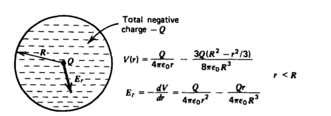
In Section 3-1-4 we modeled an atom as a fixed positive point charge nucleus Q with a surrounding uniform spherical cloud of negative charge with total charge -Q, as in Figure 3-31. Potentials due to the positive point and negative volume charges are found from Section 2-5-5b as

\[V_{+}(r) = \frac{Q}{4 \pi \varepsilon_{0}r} \\ V_{-}(r) \left \{ \begin{matrix} -\frac{3Q}{8 \pi \varepsilon_{0}R^{3}} \bigg(R^{2} - \frac{r^{2}}{3}\bigg), & r<R \\ - \frac{Q}{4 \pi \varepsilon_{0}r}, & r>R \end{matrix} \right. \]

The binding energy of the atom is easily found by superposition considering first the uniformly charged negative sphere with self-energy given in (10), (15), and (26) and then adding the energy of the positive point charge:

\[W = \frac{3Q^{2}}{20 \pi \varepsilon_{0}R} + Q[V - (r=0)] = - \frac{9Q^{2}}{40 \pi \varepsilon_{0}R} \]

This is the work necessary to assemble the atom from charges at infinity. Once the positive nucleus is in place, it attracts the following negative charges so that the field does work on the charges and the work of assembly in (31) is negative. Equivalently, the magnitude of (31) is the work necessary for us to disassemble the atom by overcoming the attractive coulombic forces between the opposite polarity charges.

When alternatively using (4) and (13), we only include the potential of the negative volume charge at r = 0 acting on the positive charge, while we include the total potential due to both in evaluating the energy of the volume charge. We do

Figure 3-31 An atom can be modelled as a point charge Q representing the nucleus, surrounded by a cloud of uniformly distributed electrons with total charge - Q within a sphere of radius R.

not consider the infinite self-energy of the point charge that would be included if we used (22):

\[W = \frac{1}{2} QV_{-}(r=0) - \frac{1}{2} \int_{r=0}^{R} [V_{+}(r) + V_{-}(r)] \frac{3Qr^{2}}{R^{3}} dr \\ = - \frac{3Q^{2}}{16 \pi \varepsilon_{0}R} - \frac{3Q^{2}}{8 \pi \varepsilon_{0}R^{3}} \int_{0}^{R} \bigg(r- \frac{3}{2} \frac{r^{2}}{R} + \frac{r^{4}}{2R^{3}}\bigg) dr \\ = - \frac{9Q^{2}}{40 \pi \varepsilon_{0}R} \]

3-8-5 Energy Stored in a Capacitor

In a capacitor all the charge resides on the electrodes as a surface charge. Consider two electrodes at voltage V₁ and V₂ with respect to infinity, and thus at voltage difference V= V₂ - V₁, as shown in Figure 3-32. Each electrode carries opposite polarity charge with magnitude Q. Then (13) can be used to compute the total energy stored as

\[W = \frac{1}{2} \bigg[ \int_{S_{1}} V_{1} \sigma_{1} dS_{1} + \int_{S_{2}} V_{2}\sigma_{2} dS_{2} \bigg] \]

Since each surface is an equipotential, the voltages V₁ and V₂ may be taken outside the integrals. The integral then reduces to the total charge \(\pm Q\) on each electrode:

\[W = \frac{1}{2} \bigg[ V_{1} \int_{S_{1}} \underbrace{\sigma_{1} dS_{1}}_{-Q} + V_{2} \int_{S_{2}} \underbrace{\sigma_{2}dS_{2}}_{Q} \bigg] = \frac{1}{2}(V_{2}-V_{1})Q = \frac{1}{2}QV \]

Figure 3-32 A capacitor stores energy in the electric field.

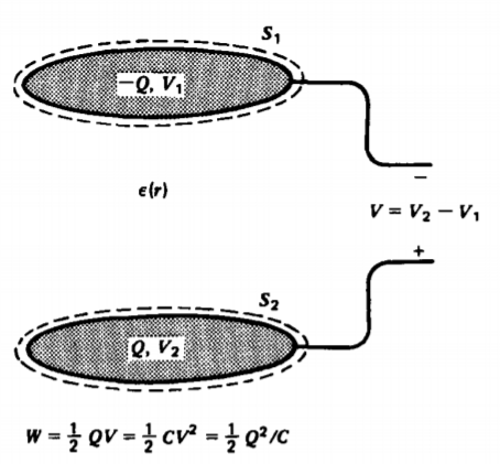
Since in a capacitor the charge and voltage are linearly related through the capacitance

\[Q = CV \]

the energy stored in the capacitor can also be written as

\[W = \frac{1}{2} QV = \frac{1}{2} CV^{2} = \frac{1}{2} \frac{Q^{2}}{C} \]

This energy is equivalent to (22) in terms of the electric field and gives us an alternate method to computing the capacitance if we know the electric field distribution.

Example 3-3: CAPACITANCE OF AN ISOLATED SPHERE

A sphere of radius R carries a uniformly distributed surface charge Q. What is its capacitance?

Answer

The stored energy is given by (28) or (29) so that (36) gives us the capacitance:

\[C = Q^{2}/2W = 4 \pi \varepsilon R \]