3.7: Field-dependent Space-Charge Distributions

A stationary Ohmic conductor with constant conductivity was shown in Section 3-6-1 to not support a steady-state volume charge distribution. This occurs because in our.classical Ohmic model in Section 3-2-2c one species of charge (e.g., electrons in metals) move relative to a stationary background species of charge with opposite polarity so that charge neutrality is maintained. However, if only one species of charge is injected into a medium, a net steady-state volume charge distribution can result.

Because of the electric force, this distribution of volume charge \(\rho_{f}\) contributes to and also in turn depends on the electric field. It now becomes necessary to simultaneously satisfy the coupled electrical and mechanical equations

3-7-1 Space Charge Limited Vacuum Tube Diode

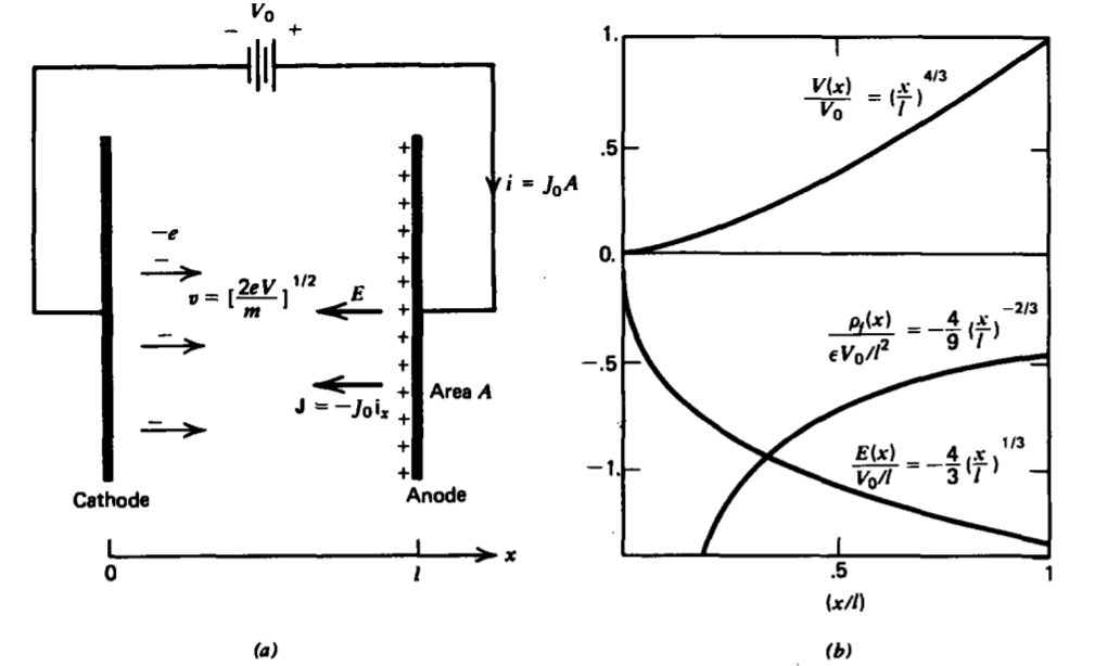
In vacuum tube diodes, electrons with charge -e and mass m are boiled off the heated cathode, which we take as our zero potential reference. This process is called thermionic emission. A positive potential V_o applied to the anode at x = l accelerates the electrons, as in Figure 3-26.

Figure 3-26 Space charge limited vacuum tube diode. (a) Thermionic injection of electrons from the heated cathode into vacuum with zero initial velocity. The positive anode potential attracts the electron whose acceleration is proportional to the local electric field. (b) Steady-state potential, electric field, and volume charge distributions.

Newton's law for a particular electron is

\[m \frac{dv}{dt} = - eE = e \frac{dV}{dx} \]

In the dc steady state the velocity of the electron depends only on its position x so that

\[m \frac{dv}{dt} = m \frac{dv}{dx} \frac{dx}{dt} = mv \frac{dv}{dx} \Rightarrow \frac{d}{dx}( \frac{1}{2} mv^{2}) = \frac{d}{dx}(eV) \]

With this last equality, we have derived the energy conservation theorem

\[\frac{d}{dx}[\frac{1}{2}mv^{2} - eV] = 0 \Rightarrow \frac{1}{2} mv^{2} - eV = \textrm{const} \]

where we say that the kinetic energy \(\frac{1}{2}mv^{2}\) plus the potential energy -eV is the constant total energy. We limit ourselves here to the simplest case where the injected charge at the cathode starts out with zero velocity. Since the potential is also chosen to be zero at the cathode, the constant in (3) is zero. The velocity is then related to the electric potential as

\[v = (\frac{2e}{m}V)^{1/2} \]

In the time-independent steady state the current density is constant,

\[\nabla \cdot \textbf{J} = 0 \Rightarrow \frac{dJ_{x}}{dx} = 0 \Rightarrow \textbf{J} = - J_{0} \textbf{i}_{x} \]

and is related to the charge density and velocity as

\[J_{0} = - \rho_{f}v \Rightarrow \rho_{f} = -J_{0}(\frac{m}{2e})^{1/2} V^{-1/2} \]

Note that the current flows from anode to cathode, and thus is in the negative x direction. This minus sign is incorporated in (5) and (6) so that Jo is positive. Poisson's equation then requires that

\[\nabla^{2}V = \frac{-\rho_{f}}{\varepsilon} \Rightarrow \frac{d^{2}V}{dx^{2}} = \frac{J_{0}}{\varepsilon}(\frac{m}{2e})^{1/2}V^{-1/2} \]

Power law solutions to this nonlinear differential equation are guessed of the form

\[V = Bx^{p} \]

which when substituted into (7) yields

\[Bp(p-1)x^{p-2} = \frac{J_{0}}{\varepsilon}(\frac{m}{2e})^{1/2}B^{-1/2} x^{-p/2} \]

For this assumed solution to hold for all x we require that

\[p-2 = -\frac{p}{2} \Rightarrow p = \frac{4}{3} \]

which then gives us the amplitude B as

\[B = \big[ \frac{9}{4} \frac{J_{0}}{\varepsilon} \big(\frac{m}{2e}\big)^{1/2} \big]^{2/3} \]

so that the potential is

\[V(x) = \big[ \frac{9}{4} \frac{J_{0}}{\varepsilon} \big( \frac{m}{2e} \big)^{1/2}\big]^{2/3} x^{4/3} \]

The potential is zero at the cathode, as required, while the anode potential Vo requires the current density to be

\[V(x=l) = V_{0} = \big[\frac{9}{4} \frac{J_{0}}{\varepsilon} \big(\frac{m}{2e} \big)^{1/2} \big]^{2/3} l^{4/3} \\ \Rightarrow J_{0} \frac{4}{9} \frac{\varepsilon}{l^{2}} \big( \frac{2e}{m} \big) ^{1/2} V_{0}^{3/2} \]

which is called the Langmuir-Child law.

The potential, electric field, and charge distributions are then concisely written as

\[V(x) = V_{0} \bigg( \frac{x}{l} \big)^{4/3} \\ E(x) = - \frac{dV(x)}{dx} = - \frac{4}{3} \frac{V_{0}}{l} \bigg( \frac{x}{l} \bigg)^{1/3} \\ \rho_{f}(x)= \varepsilon \frac{dE (x)}{dx} = - \frac{4}{9} \varepsilon \frac{V_{0}}{l^{2}} \bigg( \frac{x}{l} \bigg) ^{-2/3} \]

and are plotted in Figure 3-26b. We see that the charge density at the cathode is infinite but that the total charge between the electrodes is finite,

\[q_{\tau} = \int_{x=0}^{l} \rho_{f}(x) A \: dx = - \frac{4}{3} \varepsilon \frac{V_{0}}{l}A \]

being equal in magnitude but opposite in sign to the total surface charge on the anode:

\[q_{A} = \sigma_{f}(x=l)A = - \varepsilon E (x=l) A = + \frac{4}{3} \varepsilon \frac{V_{0}}{l}A \]

There is no surface charge on the cathode because the electric field is zero there.

This displacement x of each electron can be found by substituting the potential distribution of (14) into (4),

\[v = \frac{dx}{dt} = \bigg(\frac{2eV_{0}}{m} \bigg)^{1/2} \bigg( \frac{x}{l} \bigg)^{2/3} \Rightarrow \frac{dx}{x^{2/3}} = \bigg( \frac{2e V_{0}}{ml^{4/3}}\bigg)^{1/2} dt \]

which integrates to

\[ x=\frac{1}{27}\left(\frac{2 e V_0}{m l^{4 / 3}}\right)^{3 / 2} t^3 \]

The charge transit time \(\tau\) between electrodes is found by solving (18) with x = l :

\[\tau = 3l\bigg(\frac{m}{2eV_{0}}\bigg)^{1/2} \]

For an electron (\(m = 9.1 \times 10^{-31}\) kg, \(e = 1.6 \times 10^{-19}\) coul) with 100 volts applied across l = 1cm (10^-2 m) this time is \(\tau \approx 5 \times 10^{-9}\) sec. The peak electron velocity when it reaches the anode is \(v (x=l) \approx 6 \times 10^{6}\) m/sec, which is approximately 50 times less than the vacuum speed of light.

Because of these fast response times vacuum tube diodes are used in alternating voltage applications for rectification as current only flows when the anode is positive and as nonlinear circuit elements because of the three-halves power law of (13) relating current and voltage.

3-7-2 Space Charge Limited Conduction in Dielectrics

Conduction properties of dielectrics are often examined by injecting charge. In Figure 3-27, an electron beam with current density \(\textbf{J} = - J_{0} \textbf{i}_{x}\) is suddenly turned on at t = 0.* In media, the acceleration of the charge is no longer proportional to the electric field. Rather, collisions with the medium introduce a frictional drag so that the velocity is proportional to the electric field through the electron mobility \(\mu\):

\[\textbf{V} = \mu \textbf{E} \]

As the electrons penetrate the dielectric, the space charge front is a distance s from the interface where (20) gives us

\[ds/dt = - \mu E(s) \]

Although the charge density is nonuniformly distributed behind the wavefront, the total charge Q within the dielectric behind the wave front at time t is related to the current density as

\[J_{0}A = \rho_{f} \mu E_{x}A = -Q/t \Rightarrow Q = -J_{0}At \]

Gauss's law applied to the rectangular surface enclosing all the charge within the dielectric then relates the fields at the interface and the charge front to this charge as

\[\oint_{S} \varepsilon \textbf{E} \cdot \textbf{dS} = [\varepsilon E (s) - \varepsilon_{0}\textbf{E}(0)]A = Q = -J_{0}At \]

Figure 3-27 (a) An electron beam carrying a current \(-J_{0}\textbf{i}_{x}\) is turned on at t = 0. The electrons travel through the dielectric with mobility \(\mu\). (b) The space charge front, at a distance s in front of the space charge limited interface at x =0, travels towards the opposite electrode. (c) After the transit time \(t_{c} = [2 \varepsilon l/\mu J_{0}]^{1/2} the steady-state potential, electric field, and space charge distributions.

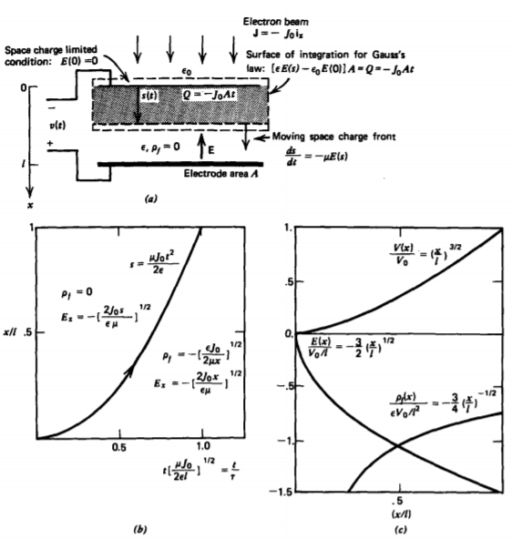
The maximum current flows when E(0) =0, which is called space charge limited conduction. Then using (23) in (21) gives us the time dependence of the space charge front:

\[\frac{ds}{dt} = \frac{\mu J_{0}t}{\varepsilon} \Rightarrow s(t) = \frac{\mu J_{0}t^{2}}{2 \varepsilon} \]

Behind the front Gauss's law requires

\[ \frac{d E_x}{d x}=\frac{\rho_f}{\varepsilon}=\frac{J_0}{\varepsilon \mu E_x} \Rightarrow E_x \frac{d E_x}{d x}=\frac{J_0}{\varepsilon \mu} \]

while ahead of the moving space charge the charge density is zero so that the current is carried entirely by displacement current and the electric field is constant in space. The spatial distribution of electric field is then obtained by integrating (25) to

\[E_{x} = \left \{ \begin{matrix} - \sqrt{2J_{0}x/\varepsilon \mu,} & 0 \leq x \leq s(t) \\ - \sqrt{2 J_{0}s/\varepsilon \mu,} & s(t) \leq x \leq l \end{matrix} \right. \]

while the charge distribution is

\[ \rho_f=\varepsilon \frac{d E_x}{d x}=\left\{\begin{array}{ll}
-\sqrt{\varepsilon J_0 /(2 \mu x)}, & 0 \leq x \leq s(t) \\
0, & s(t) \leq x \leq l
\end{array}\right. \]

as indicated in Figure 3-27b.

The time dependence of the voltage across the dielectric is then

\begin{aligned}
v(t)=\int_0^l E_x d x & =\int_0^{s(t)} \sqrt{\frac{2 J_0 x}{\varepsilon \mu}} d x+\int_{s(t)}^l \sqrt{\frac{2 J_0 s}{\varepsilon \mu}} d x \\
& =\frac{J_0 l t}{\varepsilon}-\frac{\mu J_0^2 t^3}{6 \varepsilon^2}, \quad s(t) \leq l
\end{aligned} 

\[ \]

These transient solutions are valid until the space charge front s, given by (24), reaches the opposite electrode with s = l at time

\[\tau = \sqrt{2 \varepsilon l/ \mu J_{0}} \]

Thereafter, the system is in the dc steady state with the terminal voltage V_o related to the current density as

\[J_{0} = \frac{9}{8} \frac{\varepsilon \mu V_{0}^{2}}{l^{3}} \]

which is the analogous Langmuir-Child's law for collision dominated media. The steady-state electric field and space charge density are then concisely written as

\[E_{x} = - \frac{3}{2} \frac{V_{0}}{l} \bigg( \frac{x}{l} \bigg)^{1/2}, \: \: \: \rho_{f} = \varepsilon \frac{dE}{dx} = - \frac{3}{4} \frac{\varepsilon V_{0}}{l^{2}} \bigg( \frac{x}{l} \bigg)^{-1/2} \]

and are plotted in Figure 3-27c.

In liquids a typical ion mobility is of the order of 10^-7 m²/(volt-sec) with a permittivity of \(\varepsilon = 2 \varepsilon_{0} \approx 1.77 \times 10^{-11}\) farad/m. For a spacing of l =10^-2 m with a potential difference of \(V_{0}=10^{4}V\) the current density of (30) is \(J_{0} \approx 2 \times 10^{-4}\) amp/m² with the transit time given by (29) \(\tau \approx 0.133\) sec. Charge transport times in collison dominated media are much larger than in vacuum.

* See P. K. Watson, J. M. Schneider, and H. R. Till, Electrohydrodynamic Stability of Space Charge Limited Currents In Dielectric Liquids. II. Experimental Study, Phys. Fluids 13 (1970), p. 1955.