3.6: Lossy Media

Many materials are described by both a constant permittivity \(\varepsilon\) and constant Ohmic conductivity \(\sigma\). When such a material is placed between electrodes do we have a capacitor or a resistor? We write the governing equations of charge conservation and Gauss's law with linear constitutive laws:

\[\nabla \cdot \textbf{J}_{f} + \frac{\partial \rho_{f}}{\partial t} = 0, \: \: \: \textbf{J}_{f} = \sigma \textbf{E} + \rho_{f} \textbf{U} \]

\[\nabla \cdot \textbf{D} = \rho_{f}, \: \: \: \textbf{D} = \varepsilon \textbf{E} \]

We have generalized Ohm's law in (1) to include convection currents if the material moves with velocity U. In addition to the conduction charges, any free charges riding with the material also contribute to the current. Using (2) in (1) yields a single partial differential equation in \(\rho_{f}\):

\[\sigma \underbrace{(\nabla \cdot \textbf{E})}{\rho_{f}/\varepsilon} + \nabla \cdot (\rho_{f} \textbf{U}) + \frac{\partial \rho_{f}}{\partial t} = 0 \Rightarrow \frac{\partial \rho_{f}}{\partial t} + \nabla \cdot (\rho_{f} \textbf{U}) + \frac{\sigma}{\varepsilon} \rho_{f} = 0 \]

3-6-1 Transient Charge Relaxation

Let us first assume that the medium is stationary so that U =0. Then the solution to (3) for any initial possibly spatially varying charge distribution \(\rho_{0}(x, y, z, t = 0\) is

\[\rho_{f} = \rho_{0} (x, y, z, y = 0) e^{-t/\tau}, \: \: \tau = \varepsilon/ \sigma \]

where \(\tau\) is the relaxation time. This solution is the continuum version of the resistance-capacitance (RC) decay time in circuits.

The solution of (4) tells us that at all positions within a conductor, any initial charge density dies off exponentially with time. It does not spread out in space. This is our justification of not considering any net volume charge in conducting media. If a system has no volume charge at t =0 (\(\rho_{0}=0\)), it remains uncharged for all further time. Charge is transported through the region by the Ohmic current, but the net charge remains zero. Even if there happens to be an initial volume charge distribution, for times much longer than the relaxation time the volume charge density becomes negligibly small. In metals, \(\tau\) is on the order of 10^-19 sec, which is the justification of assuming the fields are zero within an electrode. Even though their large conductivity is not infinite, for times longer than the relaxation time \(\tau\), the field solutions are the same as if a conductor were perfectly conducting.

The question remains as to where the relaxed charge goes. The answer is that it is carried by the conduction current to surfaces of discontinuity where the conductivity abruptly changes.

3-6-2 Uniformly Charged Sphere

A sphere of radius R₂ with constant permittivity \(\varepsilon\) and Ohmic conductivity \(\sigma\) is uniformly charged up to the radius R₁ with charge density \(\rho_{0}\) at time t = 0, as in Figure 3-21. From R₁ to R₂ the sphere is initially uncharged so that it remains uncharged for all time. The sphere is surrounded by free space with permittivity \(\varepsilon_{0}\) and zero conductivity.

From (4) we can immediately write down the volume charge distribution for all time,

\[\rho_{f} = \left \{ \begin{matrix} \rho_{0} e^{-t/ \tau}, & r<R_{1} \\ 0, & r>R_{1} \end{matrix} \right. \]

where \(\tau = \varepsilon / \sigma\). The total charge on the sphere remains constant, \(Q = \frac{4}{3} \pi R_{1}^{e} \rho_{0}\), but the volume charge is transported by the Ohmic current to the interface at \(r = R_{2}\) where it becomes a surface charge. Enclosing the system by a Gaussian surface with \(r > R_{2}\) shows that the external electric field is time independent,

\[E_{r} = \frac{Q}{4 \pi \varepsilon_{0}r^{2}}, \: \: \: r > R_{2} \]

Similarly, applying Gaussian surfaces for\(r < R_{1}\) and \(R_{1} < r < R_{2}\) yields

\[E_{r} = \left \{ \begin{matrix} \frac{\rho_{0}re^{-t/\tau}}{3 \varepsilon} = \frac{Qr e ^{-t/\tau}}{4 \pi \varepsilon R_{1}^{3}}, & 0 < r < R_{1} \\ \frac{Q e ^{-t/\tau}}{4 \pi \varepsilon r^{2}}, & R_{1} < r < R_{2} \end{matrix} \right. \]

Figure 3-21 An initial volume charge distribution within an Ohmic conductor decays exponentially towards zero with relaxation time \(\tau = \varepsilon/\sigma\) and appears as a surface charge at an interface of discontinuity. Initially uncharged regions are always un­ charged with the charge transported through by the current.

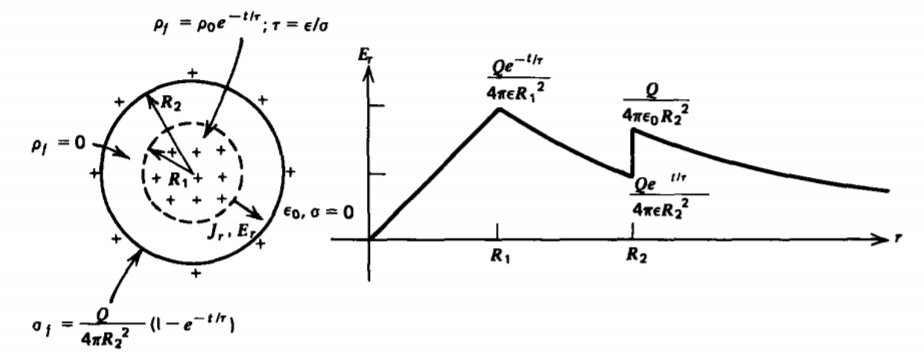
The surface charge density at r = R₂ builds up exponentially with time:

\[\sigma_{f}(r = R_{2}) = \varepsilon_{0} E_{r}(r = R_{2+}) - \varepsilon E_{r}(r = R_{2-}) = \frac{Q}{4 \pi R_{2}^{2}}(1 - e^{-t/\tau}) \]

The charge is carried from the charged region (r < R₁) to the surface at r = R₂ via the conduction current with the charge density inbetween (R₁ < r < R₂) remaining zero:

\[J_{c} = \sigma E_{r} = \left \{ \begin{matrix} \frac{\sigma Q r}{4 \pi \varepsilon R_{1}^{3}} e^{t/\tau}, & 0<r<R_{1} \\ \frac{\sigma Q e^{-t/\tau}}{4 \pi \varepsilon r^{2}}, & R_{1} < r <R_{2} \\ 0, & r >R_{2} \end{matrix} \right. \]

Note that the total current, conduction plus displacement, is zero everywhere:

\[-J_{c} = J_{d} = \varepsilon \frac{\partial E_{r}}{\partial t} = \left \{ \begin{matrix} -\frac{Qr \sigma e^{-t/\tau}}{4 \pi \varepsilon R_{1}^{3}}, & 0<r<R_{1} & - \frac{\sigma Q e^{-t/\tau}}{4 \pi \varepsilon r^{2}}, & R_{1} < r < R_{2} \\ 0, & r>R_{2} \end{matrix} \right. \]

3-6-3 Series Lossy Capacitor

(a) Charging transient

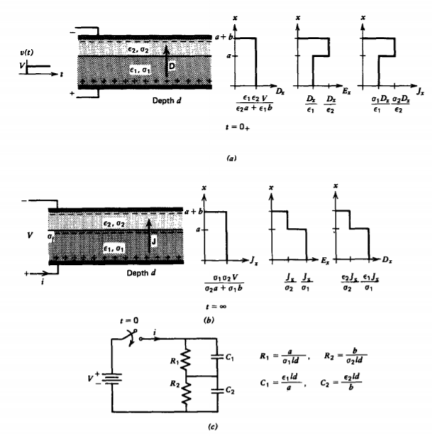
To exemplify the difference between resistive and capacitive behavior we examine the case of two different materials in series stressed by a step voltage first turned on at t =0, as shown in Figure 3-22a. Since it takes time to charge up the interface, the interfacial surface charge cannot instantaneously change at t= 0 so that it remains zero at t = 0₊. With no surface charge density, the displacement field is continuous across the interface so that the solution at t= 0₊ is the same as for two lossless series capacitors independent of the conductivities:

\[D_{x} = \varepsilon_{1}E_{1}=\varepsilon_{2}E_{2} \]

The voltage constraint requires that

\[\int_{0}^{a+b} E_{x}dx = E_{1}a + E_{2}b = V \]

Figure 3-22 Two different lossy dielectric materials in series between parallel plate electrodes have permittivities and Ohmic conductivities that change abruptly across the interface. (a) At t= 0₊, right after a step voltage is applied, the interface is uncharged so that the displacement field is continuous with the solution the same as for two lossless dielectrics in series. (b) Since the current is discontinuous across the boundary between the materials, the interface will charge up. In the dc steady state the current is continuous. (c) Each region is equivalent to a resistor and capacitor in parallel.

so that the displacement field is

\[D_{x}(t = 0_{+}) = \frac{\varepsilon_{1}\varepsilon_{2}V}{\varepsilon_{2}a + \varepsilon_{1}b} \]

The total current from the battery is due to both conduction and displacement currents. At t = 0, the displacement current is infinite (an impulse) as the displacement field instantaneously changes from zero to (13) to produce the surface charge on each electrode:

\[\sigma_{f}(x=0) = - \sigma_{f}(x = a + b) = D_{x} \]

After the voltage has been on a long time, the fields approach their steady-state values, as in Figure 3-22b. Because there are no more time variations, the current density must be continuous across the interface just the same as for two series resistors independent of the permittivities,

\[J_{x}(t \rightarrow \infty) = \sigma_{1}E_{1} = \sigma_{2}E_{2} = \frac{\sigma_{1}\sigma_{2}V}{\sigma_{2}a + \sigma_{1}b} \]

where we again used (12). The interfacial surface charge is now

\[\sigma_{f}(x=a) = \varepsilon_{2}E_{2} - \varepsilon_{1}E_{1} = \frac{(\varepsilon_{2} \sigma_{1} - \varepsilon_{1}\sigma_{2})V}{\sigma_{2}a + \sigma_{1}b} \]

What we have shown is that for early times the system is purely capacitive, while for long times the system is purely resistive. The inbetween transient interval is found by using (12) with charge conservation applied at the interface:

\[\textbf{n} \cdot (\textbf{J}_{2}-\textbf{J}_{1} + \frac{d}{dt}(\textbf{D}_{2} - \textbf{D}_{1})) = 0 \\ \Rightarrow \sigma_{2}E_{2}-\sigma_{1}E_{1} + \frac{d}{dt}[\varepsilon_{2}E_{2}-\varepsilon_{1}E_{1}]=0 \]

With (12) to relate E₂ to E₁ we obtain a single ordinary differential equation in E₁,

\[\frac{dE_{1}}{dt} + \frac{E_{1}}{\tau} = \frac{\sigma_{2}V}{\varepsilon_{2}a + \varepsilon_{1}b} \]

where the relaxation time is a weighted average of relaxation times of each material:

\[\tau = \frac{\varepsilon_{1}b + \varepsilon_{2}a}{\sigma_{1}b + \sigma_{2}a} \]

Using the initial condition of (13) the solutions for the fields are

\[E_{1} = \frac{\sigma_{2}V}{\sigma_{2}a + \sigma_{1}b}(1 - e^{-t/\tau}) + \frac{\varepsilon_{2}V}{\varepsilon_{2}a + \varepsilon_{1}b}e^{-t/\tau} \\ E_{2}= \frac{\sigma_{1}V}{\sigma_{2}a + \sigma_{1}b}(1 - e^{-t/\tau}) + \frac{\varepsilon_{1}V}{\varepsilon_{2}a + \varepsilon_{1}b}e^{-t/\tau} \]

Note that as \(t \rightarrow \infty\) the solutions approach those of (15). The interfacial surface charge is

\[\sigma_{f}(x=a) = \varepsilon_{2}E_{2} - \varepsilon_{1} E_{1} = \frac{(\varepsilon_{2}\sigma_{1} - \varepsilon_{1}\sigma_{2})}{\sigma_{2}a + \sigma_{1}b}(1 - e^{-t/\tau})V \]

which is zero at t = 0 and agrees with (16) for \(t \rightarrow \infty\).

The total current delivered by the voltage source is

\[i = (\sigma_{1}E_{1} + \varepsilon_{1}\frac{dE_{1}}{dt}) ld = (\sigma_{2}E_{2} + \varepsilon_{2} \frac{dE_{2}}{dt})ld \\ = [\frac{\sigma_{1}\sigma_{2}}{\sigma_{2}a + \sigma_{1}b} + (\sigma_{1} - \frac{\varepsilon_{1}}{\tau})(\frac{\varepsilon_{2}}{\varepsilon_{2}a + \varepsilon_{1}b} - \frac{\sigma_{2}}{\sigma_{2}a + \sigma_{1}b})e^{-t/\tau} \\ + \frac{\varepsilon_{1} \varepsilon_{2}}{\varepsilon_{2}a + \varepsilon_{1}b} \delta (t)] ldV \]

where the last term is the impulse current that instantaneously puts charge on each electrode in zero time at t =0:

\[\delta(t) = \left \{ \begin{matrix} 0, \\ t \neq 0 \\ \infty, & t = 0 \end{matrix} \right \} \infty_{0_{-}}^{0_{+}} \delta (t) dt = 1 \nonumber \]

To reiterate, we see that for early times the capacitances dominate and that in the steady state the resistances dominate with the transition time depending on the relaxation times and geometry of each region. The equivalent circuit for the system is shown in Figure 3-22c as a series combination of a parallel resistor-capacitor for each region.

(b) Open Circuit

Once the system is in the dc steady state, we instantaneously open the circuit so that the terminal current is zero. Then, using (22) with i =0, we see that the fields decay independently in each region with the relaxation time of each region:

\[E_{1} = \frac{\sigma_{2}V}{\sigma_{2}a + \sigma_{1}b} e^{-t/\tau_{1}}, \: \: \: \tau_{1} = \frac{\varepsilon_{1}}{\sigma_{1}} \\ E_{2} = \frac{\sigma_{1}V}{\sigma_{2}a + \sigma_{1}b}e^{-t/\tau_{2}}, \: \: \: \tau_{2} = \frac{\varepsilon_{2}}{\sigma_{2}} \]

The open circuit voltage and interfacial charge then decay as

\[V_{\alpha} = E_{1}a + E_{2}b = \frac{V}{\sigma_{2}a + \sigma_{1}b} [\sigma_{2}a e^{-t/\tau_{1}} + \sigma_{1} b e^{-t/\tau_{2}} \\ \sigma_{f} = \varepsilon_{2}E_{2} - \varepsilon_{1}E_{1} = \frac{V}{\sigma_{2}a + \sigma_{1}b} [\varepsilon_{2} \sigma_{1} e^{-t/\tau_{2}} - \varepsilon_{1} \sigma_{2} e^{-t/\tau_{1}}] \]

(c) Short Circuit

If the dc steady-state system is instead short circuited, we set V= 0 in (12) and (18),

\[E_{1}a + E_{2}b = 0 \\ \frac{dE_{1}}{dt} + \frac{E_{1}}{\tau} = 0 \]

where \(\tau\) is still given by (19). Since at t =0 the interfacial surface charge cannot instantaneously change, the initial fields must obey the relation

\[\lim_{t=0} (\varepsilon_{2}E_{2} - \varepsilon_{1}E_{1}) = - (\frac{\varepsilon_{2}a}{b} + \varepsilon_{1})E_{1} = \frac{(\varepsilon_{2} \sigma_{1} - \varepsilon_{1} \sigma_{2})V}{\sigma_{2}a + \sigma_{1}b} \]

to yield the solutions

\[E_{1} = - \frac{E_{2}b}{a} = - \frac{(\varepsilon_{2} \sigma_{1} - \varepsilon_{1} \sigma_{2})bV}{(\varepsilon_{2}a + \varepsilon_{1}b) (\sigma_{2}a + \sigma_{1}b)} e^{-t/\tau} \]

The short circuit current and surface charge are then

\[i = [(\frac{\sigma_{1}\varepsilon_{2} - \varepsilon_{1}\sigma_{2}}{\varepsilon_{1}b + \varepsilon_{2}a})^{2} \frac{abV}{(\sigma_{2}a + \sigma_{1}b)}e^{-t/\tau} - \frac{V \varepsilon_{1}\varepsilon_{2}}{\varepsilon_{2}a + \varepsilon_{1}b} \delta (t)] ld \\ \sigma_{f} = \varepsilon_{2}E_{2} - \varepsilon_{1}E_{1} = \frac{(\varepsilon_{2}\sigma_{1} - \varepsilon_{1} \sigma_{2})}{\sigma_{2}a + \sigma_{1} b} V e^{-t/\tau} \]

The impulse term in the current is due to the instantaneous change in displacement field from the steady-state values found from (15) to the initial values of (26).

(d) Sinusoidal Steady State Now rather than a step voltage, we assume that the applied voltage is sinusoidal,

\[v(t) = V_{0} \cos \omega t \]

and has been on a long time. The fields in each region are still only functions of time and not position. It is convenient to use complex notation so that all quantities are written in the form

\[v(t) = \textrm{Re} (V_{0}e^{j \omega t}) \\ E_{1}(t) = \textrm{Re} (\hat{E}_{1} e^{j \omega t}), \: \: \: \: E_{2}(t) = \textrm{Re}(\hat{E}_{2}e^{j \omega t}) \]

Using carets above a term to designate a complex amplitude, the applied voltage condition of (12) requires

\[\hat{E}_{1}a + \hat{E}_{2}b = V_{0} \]

while the interfacial charge conservation equation of (17) becomes

\[\sigma_{2} \hat{E}_{2} - \sigma_{1} \hat{E}_{1} + j \omega (\varepsilon_{2}\hat{E}_{2} - \varepsilon_{1}\hat{E}_{1}) = [\sigma_{2} + j \omega \varepsilon_{2}]\hat{E}_{2} - [\sigma_{1} + j \omega \varepsilon_{1}] \hat{E}_{1} = 0 \]

The solutions are

\[\frac{\hat{E}_{1}}{(j \omega \varepsilon_{2} + \sigma_{2})} = \frac{\hat{E}_{2}}{(j \omega \varepsilon_{1} + \sigma_{1})} = \frac{V_{0}}{[b(\sigma_{1} + j \omega \varepsilon_{1}) + a (\sigma_{2} + j \omega \varepsilon_{2})]} \]

which gives the interfacial surface charge amplitude as

\[\hat{\sigma}_f=\varepsilon_2 \hat{E}_2-\varepsilon_1 \hat{E}_1=\frac{\left(\varepsilon_2 \sigma_1-\varepsilon_1 \sigma_2\right) V_0}{\left[b\left(\sigma_1+j \omega \varepsilon_1\right)+a\left(\sigma_2+j \omega \varepsilon_2\right)\right]} \]

As the frequency becomes much larger than the reciprocal relaxation times,

\[\omega >> \frac{\sigma_{1}}{\varepsilon_{1}}, \: \: \: \omega >> \frac{\sigma_{2}}{\varepsilon_{2}} \]

the surface charge density goes to zero. This is because the surface charge cannot keep pace with the high-frequency alternations, and thus the capacitive component dominates. Thus, in experimental work charge accumulations can be prevented if the excitation frequencies are much faster than the reciprocal charge-relaxation times.

The total current through the electrodes is

\[\hat{I} = (\sigma_{1} + j \omega \varepsilon_{1}) \hat{E}_{1}ld = (\sigma_{2} + j \omega \varepsilon_{2}) \hat{E}_{2}ld \\ = \frac{ld(\sigma_{1} + j \omega \varepsilon_{1}) (\sigma_{2} + j \omega \varepsilon_{2}) V_{0}}{[b(\sigma_{1} + j \omega \varepsilon_{1}) + a(\sigma_{2} + j \omega \varepsilon_{2})]} \\ = \frac{V_{0}}{\frac{R_{2}}{R_{2}C_{2}j \omega + 1} + \frac{R_{1}}{R_{1}C_{1} j \omega + 1}} \]

with the last result easily obtained from the equivalent circuit in Figure 3-22c.

3-6-4 Distributed Systems

(a) Governing Equations In all our discussions we have assumed that the electrodes are perfectly conducting so that they have no resistance and the electric field terminates perpendicularly. Consider now the parallel plate geometry shown in Figure 3-23a, where the electrodes have a large but finite conductivity \(\sigma_{c}\). The electrodes are no longer equi-potential surfaces since as the current passes along the conductor an Ohmic i R drop results.

Figure 3-23 Lossy parallel plate electrodes with finite Ohmic conductivity \(\sigma_{c}\), enclose a lossy dielectric with permittivity \(\varepsilon\) and conductivity \(\sigma\). (a) This system can be modeled by a distributed resistor-capacitor network. (b) Kirchoff's voltage and current laws applied to a section of length \(\Delta z\) allow us to describe the system by partial differential equations

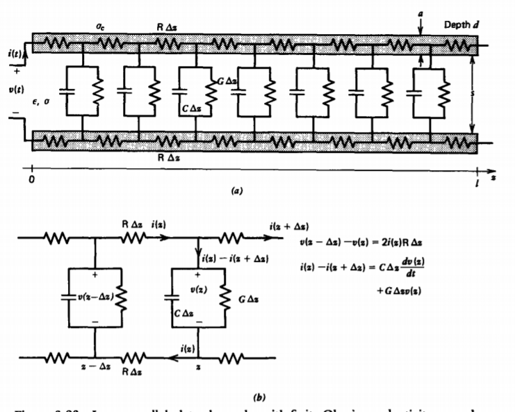
The current is also shunted through the lossy dielectric so that less current flows at the far end of the conductor than near the source. We can find approximate solutions by breaking the continuous system into many small segments of length \(\Delta z\). The electrode resistance of this small section is

\[\textrm{R} \Delta z = \frac{\Delta z}{\sigma_{c}ad} \]

where R = \(1/(\sigma_{c}ad)\) is just the resistance per unit length. We have shown in the previous section that the dielectric can be modeled as a parallel resistor-capacitor combination,

\[C \Delta z = \frac{\varepsilon d \Delta z}{s}, \: \: \frac{1}{G \Delta z} = \frac{s}{\sigma d \Delta z} \]

C is the capacitance per unit length and G is the conductance per unit length where the conductance is the reciprocal of the resistance. It is more convenient to work with the conductance because it is in parallel with the capacitance.

We apply Kirchoff's voltage and current laws for the section of equivalent circuit shown in Figure 3-23b:

\[v (z-\Delta z) - v(z) = 2 i (z) \textrm{R} \Delta z \\ i(z) - i(z + \Delta z) = C \Delta z \frac{dv(z)}{dt} + G \Delta zv (z) \]

The factor of 2 in the upper equation arises from the equal series resistances of the upper and lower conductors. Dividing through by \(\Delta z\) and taking the limit as \(\Delta z\) becomes infinitesimally small yields the partial differential equations

\[- \frac{\partial v}{\partial z} = 2i \textrm{R} \\ - \frac{\partial i}{\partial z} = C \frac{\partial v}{\partial t} + Gv \]

Taking \(\partial/ \partial z\) of the upper equation allows us to substitute in the lower equation to eliminate i,

\[\frac{\partial^{2}v}{\partial z^{2}} = 2 \textrm{R} C \frac{\partial v}{\partial t} + 2 \textrm{R} Gv \]

which is called a transient diffusion equation. Equations (40) and (41) are also valid for any geometry whose cross sectional area remains constant over its length. The 2R represents the series resistance per unit length of both electrodes, while C and G are the capacitance and conductance per unit length of the dielectric medium.

(b) Steady State

If a dc voltage V_o is applied, the steady-state voltage is

\[\frac{d^{2}v}{dz^{2}} - 2 \textrm{R} Gv = 0 \Rightarrow v = A_{1} \sinh \sqrt{2 \textrm{R} Gz} + A_{2} \cosh \sqrt{2 \textrm{R} Gz} \]

where the constants are found by the boundary conditions at z =0 and z = l,

\[v(z=0) = V_{0}, \: \: \: i(z=l) = 0 \]

We take the z = l end to be open circuited. Solutions are

\[v(z) = V_{0} \frac{\cosh \sqrt{2 \textrm{R}G}(z-l)}{\cosh \sqrt{2 \textrm{R} G} l} \\ i(z) = - \frac{1}{2 \textrm{R}} \frac{dv}{dz} = V_{0} \sqrt{\frac{G}{2 \textrm{R}}} \frac{\sinh \sqrt{2 \textrm{R}G}(z-l)}{\cosh \sqrt{2 \textrm{R} G}l} \]

(c) Transient Solution

If this dc voltage is applied as a step at t = 0, it takes time for the voltage and current to reach these steady-state distributions. Because (41) is linear, we can use superposition and guess a solution for the voltage that is the sum of the steady-state solution in (44) and a transient solution that dies off with time:

\[v(z,t) = \frac{V_{0} \cosh \sqrt{2 \textrm{R}G} (z-l)}{\cosh \sqrt{2 \textrm{R}G} l} + \hat{v}(z)e^{-\alpha t} \]

At this point we do not know the function \(\hat{v}(z)\) or \(\alpha\). Substituting the assumed solution of (45) back into (41) yields the ordinary differential equation

\[\frac{d^{2}\hat{v}}{dz^{2}} + p^{2}\hat{v} = 0, \: \: \: p^{2}=2 \textrm{R} C \alpha - 2 \textrm{R}G \]

which has the trigonometric solutions

\[\hat{v}(z) = a_{1} \sin pz + a_{2} \cos pz \]

Since the time-independent part of (45) already satisfies the boundary conditions at z =0, the transient part must be zero there so that a₂ =0. The transient contribution to the current i, found from (40),

\[i(z,t) = V_{0} \sqrt{\frac{G}{2 \textrm{R}}} \frac{\sinh \sqrt{2 \textrm{R}G} (z-l)}{\cosh \sqrt{2 \textrm{R}G} l} + \hat{i}(z) e^{-\alpha t} \\ \hat{i}(z) = - \frac{1}{2 \textrm{R}} \frac{d \hat{v}(z)}{dz} = - \frac{pa_{1}}{2 \textrm{R}} \cos pz \]

must still be zero at z = l, which means that pl must be an odd integer multiple of \(\pi\)/2,

\[pl = (2n + 1) \frac{\pi}{2} \Rightarrow \alpha_{n} = \frac{1}{2 \textrm{R} C} ((2n + 1) \frac{\pi}{2l})^{2} + \frac{G}{C}, \: \: \: \: \: n = 0,1,2... \]

Since the boundary conditions allow an infinite number of values of \(\alpha\), the most general solution is the superposition of all allowed solutions:

\[v(z,t) = V_{0} \frac{\cosh \sqrt{2 \textrm{R}G}(z-l)}{\cosh \sqrt{2 \textrm{R}G} l} + \sum_{n=0}^{\infty} A_{n} \sin (2n + 1) \frac{\pi z}{2l} e^{-\alpha_{n}t} \]

This solution satisfies the boundary conditions but not the initial conditions at t = 0 when the voltage is first turned on. Before the voltage source is applied, the voltage distribution throughout the system is zero. It must remain zero right after being turned on otherwise the time derivative in (40) would be infinite, which requires nonphysical infinite currents. Thus we impose the initial condition

\[v(z,t = 0) = 0 = V_{0} \frac{\cosh \sqrt{2 \textrm{R}G}(z-l)}{\cosh \sqrt{2 \textrm{R}G}l} + \sum_{n=0}^{\infty} A_{n} \sin (2n + 1) \frac{\pi z}{2l} \]

We can solve for the amplitudes A_n by multiplying (51) through by sin \((2m + 1) \pi z/2l\) and then integrating over z from 0 to 1:

\[0 = \frac{V_{0}}{\cosh \sqrt{2 \textrm{R}G}l} \int_{0}^{l} \cosh \sqrt{2 \textrm{R} G} (z-l) \sin (2m + 1) \frac{\pi z}{2 l} dz \\ + \int_{0}^{l} \sum_{n=0}^{\infty} A_{n} \sin (2n + 1) \frac{\pi z}{2l} \sin (2m + 1) \frac{\pi z}{2l} dz \]

The first term is easily integrated by writing the hyperbolic cosine in terms of exponentials,* while the last term integrates to zero for all values of m not equal to n so that the amplitudes are

\[A_{n} = - \frac{1}{l^{2}} \frac{\pi V_{0} (2n + 1)}{2 \textrm{R} G + [(2n + 1) \pi/2l]^{2}} \]

The total solutions are then

\[v(z,t) = \frac{V_{0} \cosh \sqrt{2 \textrm{R} G} (z-l)}{\cosh \sqrt{2 \textrm{R} G}l} \\ - \frac{\pi V_{0}}{l^{2}} \sum_{n=0}^{\infty} \frac{(2n + 1) \sin [(2n + 1)(\pi z/2l)]e^{\alpha_{n}t}}{2 \textrm{R} G + [(2n + 1) (\pi/2l)]^{2}} \\ i(z, t) = - \frac{1}{2 \textrm{R}} \frac{\partial v}{\partial z} \\ = - \frac{V_{0} \sqrt{G/2 \textrm{R}} \sinh \sqrt{2 \textrm{R}G}(z-l)}{ \cosh \sqrt{2 \textrm{R}G}l} \\ + \frac{\pi^{2} V_{0}}{4 l^{3} \textrm{R}} \sum_{n=0}^{\infty} \frac{(2n+1)^{2} \cos [(2n + 1) (\pi z/2l)]e^{-\alpha_{n}t}}{2 \textrm{R} G + [(2n + 1) ( \pi/2l)]^{2}} \]

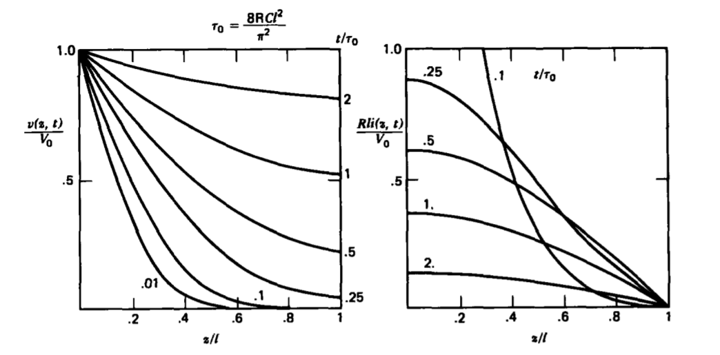
The fundamental time constant corresponds to the smallest value of \(\alpha\), which is when n = 0:

\[\tau_{0} = \frac{1}{\alpha_{0}} = \frac{C}{G + \frac{1}{2 \textrm{R}} (\frac{\pi}{2l})^{2}} \]

For times long compared to \(\tau_{0}\) the system is approximately in the steady state. Because of the fast exponential decrease for times greater than zero, the infinite series in (54) can often be approximated by the first term. These solutions are plotted in Figure 3-24 for the special case where G =0. Then the voltage distribution builds up from zero to a constant value diffusing in from the left. The current near z =0 is initially very large. As time increases, with G =0, the current everywhere decreases towards a zero steady state.

* \(\int \cosh a(z-l) \sin bz \: dz \\ = \frac{1}{a^{2} + b^{2}} [a \sin \: bz \: \sinh \: a(z-l) - b \cos \: bh \cosh \: a(z-l)] \\ \int_{0}^{l} \sin (2n+1) bz \sin(2m+1) bz \: dz = \left \{ \begin{matrix} 0 & m \neq n \\ l/2 & m=n \end{matrix} \right.\)

3-6-5 Effects of Convection

We have seen that in a stationary medium any initial charge density decays away to a surface of discontinuity. We now wish to focus attention on a dc steady-state system of a conducting medium moving at constant velocity U i_x, as in Figure 3-25. A source at x =0 maintains a constant charge density \(\rho_{0}\). Then (3) in the dc steady state with constant

Figure 3-23a with G = 0 for a step voltage excitation at z = 0 with the z = l end open circuited. The diffusion effects arise because of the lossy electrodes where the longest time constant is \(\tau_{0} = 8 \textrm{R} Cl^{2}/\pi^{2}\).

Figure 3-25 A moving conducting material with velocity U i_x tends to take charge injected at x =0 with it. The steady-state charge density decreases exponentially from the source

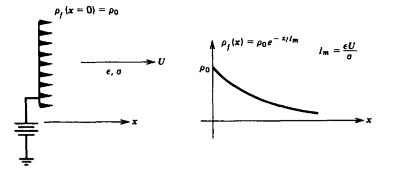
velocity becomes

\[\frac{d \rho_{f}}{dx} + \frac{\sigma}{\varepsilon U} \rho_{f} = 0 \]

which has exponentially decaying solutions

\[\rho_{f} = \rho_{0} e^{-x/l_{m}}, \: \: \: \: l_{m} = \frac{\varepsilon U}{\sigma} \]

where l_m, represents a characteristic spatial decay length. If the system has cross-sectional area A, the total charge q in the system is

\[q = \int_{0}^{\infty} \rho_{f}A \: dx = \rho_{0} l_{m}A \]

3-6-6 The Earth and its Atmosphere as a Leaky Spherical Capacitor*

In fair weather, at the earth's surface exists a dc electric field with approximate strength of 100 V/m directed radially toward the earth's center. The magnitude of the electric field decreases with height above the earth's surface because of the nonuniform electrical conductivity \(\sigma(r)\) of the atmosphere approximated as

\[\sigma(r) = \sigma_{0} + a(r-R)^{2} \textrm{siemen/m} \]

where measurements have shown that and R ~6 x 106 meter is the earth's radius. The conductivity increases with height because of cosmic radiation in the lower atmosphere. Because of solar radiation the atmosphere acts as a perfect conductor above 50 km

\[\sigma_{0} \approx 3 \times 10^{-14} \\ a \approx .5 \times 10^{-20} \]

In the dc steady state, charge conservation of Section 3-2-1 with spherical symmetry requires

\[\nabla \cdot \textbf{J} = \frac{1}{r^{2}} \frac{\partial}{\partial r} (r^{2}J_{r}) = 0 \Rightarrow J_{r} = \sigma(r)E_{r} = \frac{C}{r^{2}} \]

where the constant of integration C is found by specifying the surface electric field \(E_{r} (R) \approx -100\) V/m

\[J_{r}(r) = \frac{\sigma(R)_{r}(R)R^{2}}{r^{2}} \]

At the earth's surface the current density is then

\[ J_r(R)=\sigma(R) E_r(R)=\sigma_0 E_r(R) \approx-3 \times 10^{-12} \mathrm{amp} / \mathrm{m}^2 \]

The total current directed radially inwards over the whole earth is then

\[I = \vert J_{r}(R) 4 \pi R^{2} \vert \approx 1350 \textrm{ amp} \]

The electric field distribution throughout the atmosphere is found from (62) as

\[E_{r}(R) = \frac{J_{r}(r)}{\sigma(r)} = \frac{\sigma(R)E_{r}(R)R^{2}}{r^{2}\sigma(r)} \]

The surface charge density on the earth's surface is

\[\sigma_{f}(r=R) = \sigma_{0}E_{r}(R) \approx - 8.85 \times 10^{-10} \textrm{Coul/m}^{2} \]

This negative surface charge distribution (remember: E_r(r) < 0) is balanced by positive volume charge distribution throughout the atmosphere

\[\rho_{f}(r) = \varepsilon_{0} \nabla \cdot \textbf{E} = \frac{\varepsilon_{0}}{r^{2}}\frac{\partial}{\partial r}(r^{2} E_{r}) = \frac{\varepsilon_{0} \sigma (R) E_{r}(R) R^{2}}{r^{2}} \frac{d}{dr} (\frac{1}{\sigma(r)}) \\ = \frac{- \varepsilon_{0} \sigma(R) E_{r}(R) R^{2}}{r^{2}(\sigma(r))^{2}}2a(r-R) \]

The potential difference between the upper atmosphere and the earth's surface is

\[V = - \int_{R}^{\infty} E_{r}(r)dr \\ = - \sigma (R)E_{r}(R)R^{2} \int_{R}^{\infty} \frac{dr}{r^{2}[\sigma_{0} + a(r-R)^{2}]} \\ = - \frac{\sigma(R)E_{r}(R)R^{2}}{a} \left \{ \begin{matrix} - \frac{R}{(R^{2} + \frac{\sigma_{0}}{a})^{2}} \ln \big[\frac{(r-R)^{2} + \frac{\sigma_{0}}{a}}{r^{2}}\big] - \frac{1}{r(R^{2} + \frac{\sigma_{0}}{a})} + \frac{(R^{2} - \frac{\sigma_{0}}{a})}{\sqrt{\frac{\sigma_{0}}{a}}(R^{2} + \frac{\sigma_{0}}{a})^{2}} \tan^{-1} \frac{(r-R)}{\sqrt{\frac{\sigma_{0}}{a}}} \end{matrix} \right \} \Bigg|_{r+R}^{\infty} \\ = - \frac{\sigma(R)E_{r}(R)}{a(R^{2} + \frac{\sigma_{0}}{a})^{2}}R^{2} \left \{ \begin{matrix} R \ln \frac{\sigma_{0}}{aR^{2}} + \frac{(R^{2} + \frac{\sigma_{0}}{a})}{R} + \frac{\frac{\pi}{2}(R^{2} - \frac{\sigma_{0}}{a})}{\sqrt{\frac{\sigma_{0}}{a}}} \end{matrix} \right \} \]

Using the parameters of (60), we see that \(\sigma_{0}/a << R^{2}\) so that (68) approximately reduces to

\[V \approx - \frac{\sigma_{0}E_{r}(R)}{aR^{2}} \left \{ \begin{matrix} R \big(\ln \frac{\sigma_{0}}{a R^{2}} + 1 \big) + \frac{\pi R^{2}}{2 \sqrt{\frac{\sigma_{0}}{a}}} \end{matrix} \right \} \\ \approx 384,000 \textrm{volts} \]

If the earth's charge were not replenished, the current flow would neutralize the charge at the earth's surface with a time constant of order

\[\tau = \frac{\varepsilon_{0}}{\sigma_{0}} \approx 300 \textrm{ seconds} \]

It is thought that localized stormy regions simultaneously active all over the world serve as "batteries" to keep the earth charged via negatively chariged lightning to ground and corona at ground level, producing charge that moves from ground to cloud. This thunderstorm current must be upwards and balances the downwards fair weather current of (64).

* M. A. Uman, "The EarthandIts Atmosphere asa Leaky SphericalCapacitor,"Am. J. Phys. V. 42, Nov. 1974, pp. 1033-1035.