3.5: Capacitance

Parallel Plate Electrodes

Parallel plate electrodes of finite size constrained to potential difference v enclose a dielectric medium with permittivity \(\varepsilon\). The surface charge density does not distribute itself uniformly, as illustrated by the fringing field lines for infinitely thin parallel plate electrodes in Figure 3-17a. Near the edges the electric field is highly nonuniform decreasing in magnitude on the back side of the electrodes. Between the electrodes, far from the edges the electric field is uniform, being the same as if the electrodes were infinitely long. Fringing field effects can be made negligible if the electrode spacing l is much less than the depth d or width w. For more accurate work, end effects can be made even more negligible by using a guard ring encircling the upper electrode, as in Figure 3-17b. The guard ring is maintained at the same potential as the electrode, thus except for the very tiny gap, the field between

Figure 3-17 (a) Two infinitely thin parallel plate electrodes of finite area at potential difference v have highly nonuniform fields outside the interelectrode region. (b) A guard ring around one electrode removes end effects so that the field between the electrodes is uniform. The end effects now arise at the edge of the guard ring, which is far from the region of interest.

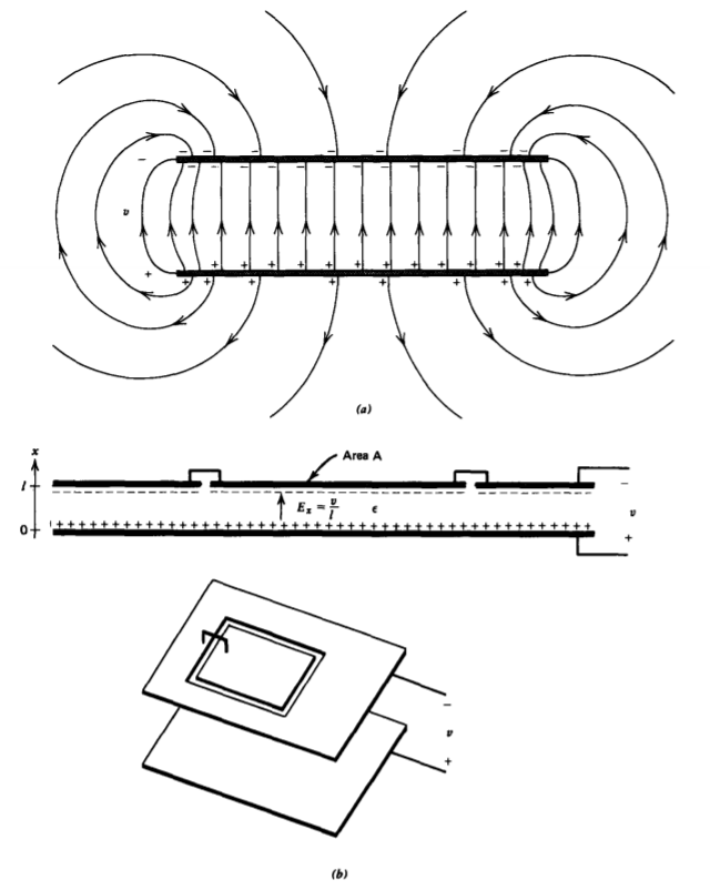
the electrodes is as if the end effects were very far away and not just near the electrode edges.

We often use the phrase "neglect fringing" to mean that the nonuniform field effects near corners and edges are negligible.

With the neglect of fringing field effects near the electrode ends, the electric field is perpendicular to the electrodes and related to the voltage as

\[\int_{0}^{l} E_{x}dx = v \Rightarrow E_{x} = v/l \]

The displacement vector is then proportional to the electric field terminating on each electrode with an equal magnitude but opposite polarity surface charge density given by

\[D_{x} = \varepsilon E_{x} = \sigma_{f}(x=0) = - \sigma_{F}(x = l) = \varepsilon v/l \]

The charge is positive where the voltage polarity is positive, and vice versa, with the electric field directed from the positive to negative electrode. The magnitude of total free charge on each electrode is

\[q_{f} = \sigma_{f} (x = 0)A = \frac{\varepsilon A}{l} v \]

The capacitance C is defined as the magnitude of the ratio of total free charge on either electrode to the voltage difference between electrodes:

\[C = \frac{q_{f}}{v} = \frac{\varepsilon A}{l} = \frac{\textrm{(permittivity)(electrode area)}}{\textrm{spacing}} \textrm{farad}[\textrm{A}^{2} \textrm{s}^{4} \textrm{kg}^{-1} \textrm{m}^{-2}] \]

Even though the system remains neutral, mobile electrons on the lower electrode are transported through the voltage source to the upper electrode in order to terminate the displacement field at the electrode surfaces, thus keeping the fields zero inside the conductors. Note that no charge is transported through free space. The charge transport between electrodes is due to work by the voltage source and results in energy stored in the electric field.

In SI units, typical capacitance values are very small. If the electrodes have an area of A = 1 cm² (10^-4 m²) with spacing of l = 1 mm (10^-3 m), the free space capacitance is \(C \approx 0.9 \times 10^{-12}\) farad. For this reason usual capacitance values are expressed in microfarads (1 \(\mu\) f = 10^-6 farad), nanofarads (1 nf = 10^-9 farad), and picofarads (1 pf = 10^-12 farad).

With a linear dielectric of permittivity \(\varepsilon\) as in Figure 3-18a, the field of (1) remains unchanged for a given voltage but the charge on the electrodes and thus the capacitance increases with the permittivity, as given by (3). However, if the total free charge on each electrode were constrained, the voltage difference would decrease by the same factor.

These results arise because of the presence of polarization charges on the electrodes that partially cancel the free charge. The polarization vector within the dielectric-filled parallel plate capacitor is a constant

\[P_{x} = D_{x} - \varepsilon_{0}E_{x} = (\varepsilon - \varepsilon_{0}) E_{x} = (\varepsilon - \varepsilon_{0}) v/l \]

so that the volume polarization charge density is zero. However, with zero polarization in the electrodes, there is a discontinuity in the normal component of polarization at the electrode surfaces. The boundary condition of Section 3.3.4 results in an equal magnitude but opposite polarity surface polarization charge density on each electrode, as illustrated in

Figure 3-18 The presence of a dielectric between the electrodes increases the capacitance because for a given voltage additional free charge is needed on each electrode to overcome the partial neutralization of the attracted opposite polarity dipole ends. (a) Parallel plate electrodes. (b) Coaxial cylinders. (c) Concentric spheres.

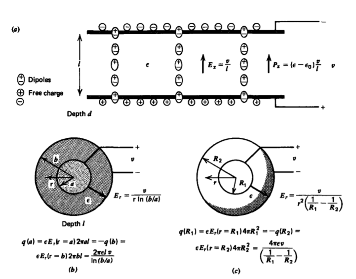
Figure 3-18a:

\[\sigma_{p} (x=0) = -\sigma_{p} (x=l) = - P_{x} = - (\varepsilon - \varepsilon_{0}) v/l \]

Note that negative polarization charge appears on the positive polarity electrode and vice versa. This is because opposite charges attract so that the oppositely charged ends of the dipoles line up along the electrode surface partially neutralizing the free charge.

3-5-2 Capacitance for any Geometry

We have based our discussion around a parallel plate capacitor. Similar results hold for any shape electrodes in a dielectric medium with the capacitance defined as the magnitude of the ratio of total free charge on an electrode to potential difference. The capacitance is always positive by definition and for linear dielectrics is only a function of the geometry and dielectric permittivity and not on the voltage levels,

\[C = \frac{q_{f}}{v} = \frac{\oint_{S} \textbf{D} \cdot \textbf{dS}}{\int_{L} \textbf{E} \cdot \textbf{dl}} = \frac{\oint_{S} \varepsilon \textbf{E} \cdot \textbf{dS}}{\int_{L} \textbf{E} \cdot \textbf{dl}} \]

as multiplying the voltage by a constant factor also increases the electric field by the same factor so that the ratio remains unchanged.

The integrals in (7) are similar to those in Section 3.4.1 for an Ohmic conductor. For the same geometry filled with a homogenous Ohmic conductor or a linear dielectric, the resistance-capacitance product is a constant independent of the geometry:

\[\textrm{R} C = \frac{\int_{L} \textbf{E} \cdot \textbf{dl}}{\sigma \oint_{S} \textbf{E} \cdot \textbf{dS}} \frac{\varepsilon \oint_{S} \textbf{E} \cdot \textbf{dS}}{\int_{L} \textbf{E} \cdot \textbf{dl}} = \frac{\varepsilon}{\sigma} \]

Thus, for a given geometry, if either the resistance or capacitance is known, the other quantity is known immediately from (8). We can thus immediately write down the capacitance of the geometries shown in Figure 3-18 assuming the medium between electrodes is a linear dielectric with permittivity e using the results of Sections 3.4.2-3.4.4:

\[\textrm{Parallel Plate R} = \frac{l}{\sigma A} \Rightarrow C = \frac{\varepsilon A}{l} \\ \textrm{Coaxial R} = \frac{\ln (b/a)}{2 \pi \sigma l} \Rightarrow C = \frac{2 \pi \varepsilon l}{\ln (b/a)} \\ \textrm{Spherical R} = \frac{1/R_{1} - 1/R_{2}}{4 \pi \sigma} \Rightarrow C = \frac{4 \pi \varepsilon}{(1/R_{1} - 1/R_{2})} \]

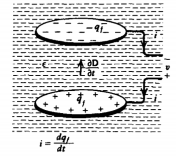
3-5-3 Current Flow Through a Capacitor

From the definition of capacitance in (7), the current to an electrode is

\[i = \frac{dq_{f}}{dt} = \frac{d}{dt} (Cv) = C \frac{dv}{dt} + v \frac{dC}{dt} \]

where the last term only arises if the geometry or dielectric permittivity changes with time. For most circuit applications, the capacitance is independent of time and (10) reduces to the usual voltage-current circuit relation.

In the capacitor of arbitrary geometry, shown in Figure 3-19, a conduction current i flows through the wires into the upper electrode and out of the lower electrode changing the amount of charge on each electrode, as given by (10). There is no conduction current flowing in the dielectric between the electrodes. As discussed in Section 3.2.1 the total current, displacement plus conduction, is continuous. Between the electrodes in a lossless capacitor, this current is entirely displacement current. The displacement field is itself related to the time-varying surface charge distribution on each electrode as given by the boundary condition of Section 3.3.2.

3-5-4 Capacitance of Two Contacting Spheres

If the outer radius R₂ of the spherical capacitor in (9) is put at infinity, we have the capacitance of an isolated sphere of radius R as

\[C = 4 \pi \varepsilon R \]

Figure 3-19 The conduction current i that travels through the connecting wire to an electrode in a lossless capacitor is transmitted through the dielectric medium to the opposite electrode via displacement current. No charge carriers travel through the lossless dielectric.

If the surrounding medium is free space (\(\varepsilon = \varepsilon_{0}\)) for R = 1 m, we have that \(C \approx \frac{1}{9} \times 10^{-9}\) farad \(\approx\) 111 pf.

We wish to find the self-capacitance of two such contacting spheres raised to a potential V_o, as shown in Figure 3-20. The capacitance is found by first finding the total charge on the two spheres. We can use the method of images by first placing an image charge \(q_{1} = Q = 4 \pi \varepsilon R V_{0}\) at the center of each sphere to bring each surface to potential V_o. However, each of these charges will induce an image charge q₂ in the other sphere at distance b₂ from the center,

\[q_{2} = - \frac{Q}{2}, \: \: \: \: b_{2} = \frac{R^{2}}{D} = \frac{R}{2} \]

where we realize that the distance from inducing charge to the opposite sphere center is D = 2R. This image charge does not raise the potential of either sphere. Similarly, each of these image charges induces another image charge q₃ in the other sphere at distance b₃

\[Q_{3} = - \frac{q_{2}R}{D-b_{2}} = \frac{Q}{3}, \: \: \: \: b_{3} = \frac{R^{2}}{D-b_{2}} = \frac{2}{3}R \]

which will induce a further image charge q₄, ad infinitum. An infinite number of image charges will be necessary, but with the use of difference equations we will be able to add all the image charges to find the total charge and thus the capacitance.

The nth image charge q_n and its distance from the center b_n are related to the (n - 1)th images as

\[q_{n} = - \frac{q_{n-1}R}{D-b_{n-1}}, \: \: \: \: b_{n} = \frac{R^{2}}{D-b_{n-1}} \]

Figure 3-20 Two identical contacting spheres raised to a potential V_O with respect to infinity are each described by an infinite number of image charges q_n each a distance b_n from the sphere center.

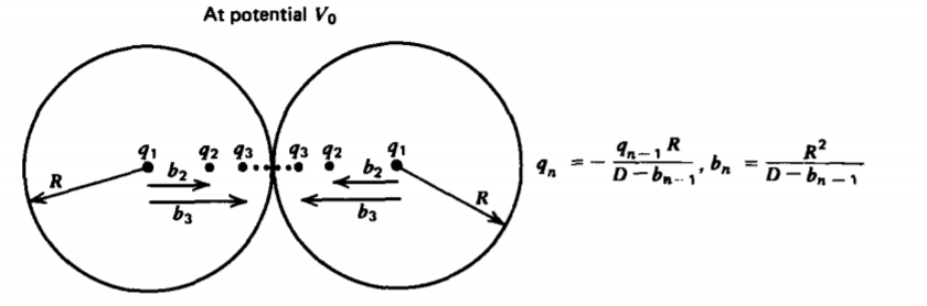
where D = 2R. We solve the first relation for b_n-1 as

\[D - b_{n-1} = - \frac{q_{n-1}}{q_{n}} R \\ b_{n} = \frac{q_{n}}{q_{n+1}} R + D \]

where the second relation is found by incrementing n in the first relation by 1. Substituting (15) into the second relation of (14) gives us a single equation in the q_n's:

\[\frac{q_{n}R}{q_{n+1}} + D = - \frac{Rq_{n}}{q_{n-1}} \Rightarrow \frac{1}{q_{n+1}} + \frac{2}{q_{n}} + \frac{1}{q_{n-1}} = 0 \]

If we define the reciprocal charges as

\[p_{n} = 1/q_{n} \]

then (16) becomes a homogeneous linear constant coefficient difference equation

\[p_{n+1} + 2 p_{n} + p_{n-1} = 0 \]

Just as linear constant coefficient differential equations have exponential solutions, (18) has power law solutions of the form

\[p_{n} = A \lambda^{n} \]

where the characteristic roots \(\lambda\), analogous to characteristic frequencies, are found by substitution back into (18),

\[\lambda^{n+1} + 2 \lambda^{n} + \lambda^{n-1} = 0 \Rightarrow \lambda^{2} + 2 \lambda + 1 = (\lambda + 1)^{2} = 0 \]

to yield a double root with \(\lambda\) = -1. Because of the double root, the superposition of both solutions is of the form

\[p_{n} = A_{1}(-1)^{n} + A_{2}n(-1)^{n} \]

similar to the behavior found in differential equations with double characteristic frequencies. The correctness of (21) can be verified by direct substitution back into (18). The constants A₁ and A₂ are determined from q₁ and q₂ as

\[\left. \begin{matrix} P_{1} = 1/Q = -A_{1} -A_{2} \\ p_{2} = \frac{1}{q_{2}} = - \frac{2}{Q} = + A_{1} + 2A_{2} \end{matrix} \right \} \Rightarrow \left \{ \begin{matrix} A_{1} = 0 \\ A_{2} = - \frac{1}{Q} \end{matrix} \right. \]

so that the nth image charge is

\[q_{n} = \frac{1}{p_{n}} = \frac{1}{-(-1)^{n} n/Q} = \frac{-(-1)^{n}Q}{n} \]

The capacitance is then given as the ratio of the total charge on the two spheres to the voltage,

\[C = \frac{2 \sum_{n=0}^{\infty} q_{n}}{V_{0}} = - \frac{2Q}{V_{0}} \sum_{n=1}^{\infty} \frac{(-1)^{n}}{n} = + \frac{2Q}{V_{0}}[1 - \frac{1}{2} + \frac{1}{3} - \frac{1}{4} + ...\\ = 8 \pi \varepsilon R \ln 2 \]

where we recognize the infinite series to be the Taylor series expansion of ln (1 + x) with x = 1. The capacitance of two contacting spheres is thus \(2 \ln 2 \approx 1.39\) times the capacitance of a single sphere given by (11).

The distance from the center to each image charge is obtained from (23) substituted into (15) as

\[b_{n} = (\frac{(-1)^{n} (n + 1)}{n (-1)^{n+1}} + 2 ) R = \frac{(n-1)}{n}R \]

We find the force of attraction between the spheres by taking the sum of the forces on each image charge on one of the spheres due to all the image charges on the other sphere. The force on the nth image charge on one sphere due to the mth image charge in the other sphere is

\[f_{nm} = \frac{-q_{n}q_{m}}{4 \pi \varepsilon [2R - b_{n} - b_{m}]^{2}} = \frac{-Q^{2}_{0}(-1)^{n+m}}{4 \pi \varepsilon R^{2}} \frac{nm}{(m + n)^{2}} \]

where we used (23) and (25). The total force on the left sphere is then found by summing over all values of m and n,

\[f = \sum_{m=1}^{\infty} \sum_{n=1}^{\infty} f_{nm} = \frac{-Q_{0}^{2}}{4 \pi \varepsilon R^{2}} \sum_{m=1}^{\infty} \sum_{n=1}^{\infty} \frac{(-1)^{n+m}nm}{(n+m)^{2}} \\ = \frac{-Q_{0}^{2}}{4 \pi \varepsilon R^{2}} \frac{1}{6} [\ln 2 - \frac{1}{4}] \]

where the double series can be explicitly expressed.* The force is negative because the like charge spheres repel each other. If Q_o = 1 coul with R = 1 m, in free space this force is \(f \approx 6.6 \times 10^{8}\) nt, which can lift a mass in the earth's gravity field of 6.8 x 10⁷ kg (\(\approx \times 10^{7}\) lb).

* See Albert D. Wheelon, Tables of Summable Series and Integrals Involving Bessel Functions, Holden Day, (1968) pp. 55, 56.