4.2: Boundary Value Problems in Cartesian Geometries

For most of the problems treated in Chapters 2 and 3 we restricted ourselves to one-dimensional problems where the electric field points in a single direction and only depends on that coordinate. For many cases, the volume is free of charge so that the system is described by Laplace's equation. Surface charge is present only on interfacial boundaries separating dissimilar conducting materials. We now consider such volume charge-free problems with two- and three dimensional variations.

4-2-1 Separation of Variables

Let us assume that within a region of space of constant permittivity with no volume charge, that solutions do not depend on the z coordinate. Then Laplace's equation reduces to

\[\frac{\partial^{2}V}{\partial x^{2}} + \frac{\partial^{2}V}{\partial y^{2}} = 0 \]

We try a solution that is a product of a function only of the x coordinate and a function only of y:

\[V(x,y) = X (x) Y(y) \]

This assumed solution is often convenient to use if the system boundaries lay in constant x or constant y planes. Then along a boundary, one of the functions in (2) is constant. When (2) is substituted into (1) we have

\[Y \frac{d^{2}X}{dx^{2}} + X \frac{d^{2}Y}{dy^{2}} = 0 \Rightarrow \frac{1}{X} \frac{d^{2}X}{dx^{2}} + \frac{1}{Y} \frac{d^{2}Y}{dy^{2}} = 0 \]

where the partial derivatives become total derivatives because each function only depends on a single coordinate. The second relation is obtained by dividing through by XY so that the first term is only a function of x while the second is only a function of y.

The only way the sum of these two terms can be zero for all values of x and y is if each term is separately equal to a constant so that (3) separates into two equations,

\[\frac{1}{X} \frac{d^{2}X}{dx^{2}} = k^{2}, \: \: \: \frac{1}{Y} \frac{d^{2}Y}{dy^{2}} = -k^{2} \]

where k² is called the separation constant and in general can be a complex number. These equations can then be rewritten as the ordinary differential equations:

\[\frac{d^{2}X}{dx^{2}} - k^{2}X = 0, \: \: \: \: \frac{d^{2} Y}{dy^{2}} + k^{2} Y =0 \]

4-2-2 Zero Separation Constant Solutions

When the separation constant is zero (k² =0) the solutions to (5) are

\[X = a_{1}x + b_{1}, \: \: \: \: Y = c_{1}y + d_{1} \]

where a₁, b₁, c₁, and d₁ are constants. The potential is given by the product of these terms which is of the form

\[V = a_{2} + b_{2}x + c_{2}y + d_{2}xy \]

The linear and constant terms we have seen before, as the potential distribution within a parallel plate capacitor with no fringing, so that the electric field is uniform. The last term we have not seen previously.

(a) Hyperbolic Electrodes

A hyperbolically shaped electrode whose surface shape obeys the equation xy = ab is at potential V_o and is placed above a grounded right-angle corner as in Figure 4-1. The

Figure 4-1 The equipotential and field lines for a hyperbolically shaped electrode at potential V_o above a right-angle conducting corner are orthogonal hyperbolas.

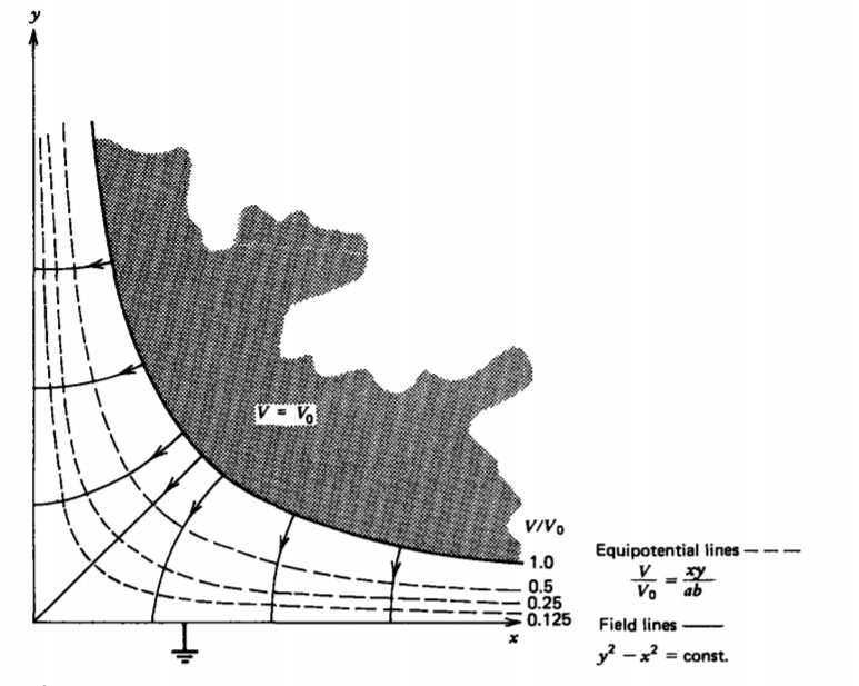
boundary conditions are

\[V(x=0) = 0, \: \: \: \: V(y=0) = 0, \: \: \: V(y=0) = 0, \: \: \: \: V(xy=ab) = V_{0} \]

so that the solution can be obtained from (7) as

\[V (x,y) = V_{0} xy/(ab) \]

The electric field is then

\[\textbf{E} = - \nabla V = - \frac{V_{0}}{ab}[y \textbf{i}_{x} + x \textbf{i}_{y}] \]

The field lines drawn in Figure 4-1 are the perpendicular family of hyperbolas to the equipotential hyperbolas in (9):

\[\frac{dy}{dx} = \frac{E_{y}}{E_{x}} = \frac{x}{y} \Rightarrow y^{2} - x^{2} = \textrm{const} \]

(b) Resistor in an Open Box

A resistive medium is contained between two electrodes, one of which extends above and is bent through a right-angle corner as in Figure 4-2. We try zero separation constant

Figure 4-2: A resistive medium partially fills an open conducting box

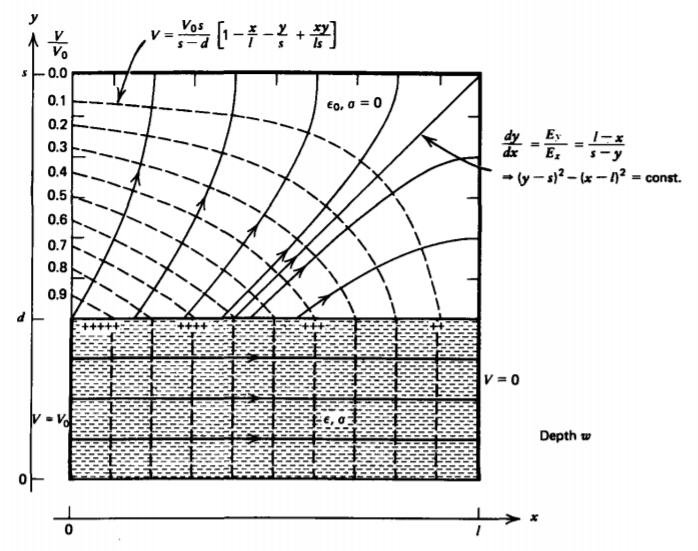
solutions given by (7) in each region enclosed by the electrodes:

\[V = \left \{ \begin{matrix} a_{1} + b_{1} x + c_{1} y + d_{1}xy, & 0 \leq y \leq d \\ a_{2} + b_{2}x + c_{2}y + d_{2}xy, & d \leq y \leq s \end{matrix} \right. \]

With the potential constrained on the electrodes and being continuous across the interface, the boundary conditions are

\[V (x=0) = V_{0} = a_{1} + C_{1}y \Rightarrow a_{1} = V_{0}, \: \: \: c_{1} = 0 \: \: \: \: \: \: (0 \leq y \leq d) \\ V(x=l) = 0 = \left \{ \begin{matrix} \underbrace{a_{1}}_{V_{0}} + b_{1} l + c_{1} \nearrow^{0} y + d_{1} ly \Rightarrow b_{1} = - V_{0}/l, & d_{1}=0 & (0 \leq y \leq d) \\ a_{2} +b_{2}l + c_{2}y + d_{2} ly \Rightarrow a_{2} + b_{2}l = 0, & c_{2} + d_{2}l = 0 & (d \leq y \leq s) \end{matrix} \right. \\ V(y=s) = 0 = a_{2} + b_{2}x + c_{2}s + d_{2} xs \Rightarrow a_{2} + c_{2}s = 0, \: \: \: b_{2} + d_{2}s = 0 \\ V(y = d_{+}) = V (y = d_{-}) = a_{1} + b_{1}x + c \nearrow^{0} d + d \nearrow^{0}_{1} xd \\ = a_{2} + b_{2}x + c_{2}d + d_{2} xd \\ \Rightarrow a_{1} = V_{0} = a_{2} + c_{2}d, \: \: \: b_{1} = -V_{0}/l = b_{2} + d_{2}d \]

so that the constants in (12) are

\[a_{1}=V_{0}, \: \: \: \: b_{1} = -V_{0}/l, \: \: \: \: c_{1} = 0, \: \: \: \: d_{1} = 0 \\ a_{2} = \frac{V_{0}}{(1-d/s)}, \: \: \: \: b_{2} = - \frac{V_{0}}{l(1-d/s)}, \\ c_{2} = - \frac{V_{0}}{s(1-d/s)}, \: \: \: \: d_{2} = \frac{V_{0}}{ls(1-d/s)} \]

The potential of (12) is then

\[V = \left \{ \begin{matrix} V_{0} (1-x/l), & 0 \leq y \leq d \\ \frac{V_{0}s}{s-d} \bigg(1 - \frac{x}{l} - \frac{y}{s} + \frac{xy}{ls} \bigg), & d \leq y \leq s \end{matrix} \right. \]

with associated electric field

\[\textbf{E} = - \nabla V = \left \{ \begin{matrix} \frac{V_{0}}{l} \textbf{i}_{x}, & 0 \leq y \leq d \\ \frac{V_{0}s}{s-d} \bigg[ \frac{\textbf{i}_{x}}{l} \bigg( 1 - \frac{y}{s} \bigg) + \frac{\textbf{i}_{y}}{s} \bigg(1 - \frac{x}{l} \bigg) \bigg], & d<y<s \end{matrix} \right. \]

Note that in the dc steady state, the conservation of charge boundary condition of Section 3-3-5 requires that no current cross the interfaces at y = 0 and y = d because of the surrounding zero conductivity regions. The current and, thus, the electric field within the resistive medium must be purely tangential to the interfaces, E,(y=d..)=E,(y=0+)=0. The surface charge density on the interface at y = d is then due only to the normal electric field above, as below, the field is purely tangential:

\[\sigma_{f}(y=d) = \varepsilon_{0}E_{y}(y = d_{+}) - \varepsilon E_{y} \nearrow^{0} (y = d_{-}) = \frac{\varepsilon_{0}V_{0}}{s-d} \bigg(1-\frac{x}{l} \bigg) \]

The interfacial shear force is then

\[F_{x} = \int_{0}^{l} \sigma_{f}E_{x}(y=d)w \: dx = \frac{\varepsilon_{0} V_{0}^{2}}{2(s-d)} w \]

If the resistive material is liquid, this shear force can be used to pump the fluid.*

4-2-3 Nonzero Separation Constant Solutions

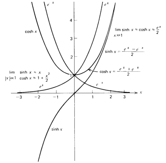
Further solutions to (5) with nonzero separation constant (\(k^{2} \neq 0\)) are

\[X = A_{1} \sinh kx + A_{2} \cosh kx = B_{1} e^{kx} + B_{2} e^{-kx} \\ Y = C_{1} \sin ky + C_{2} \cos ky = D_{1} e^{jky} + D_{2} e^{-jky} \]

When k is real, the solutions of X are hyperbolic or equivalently exponential, as drawn in Figure 4-3, while those of Y are trigonometric. If k is pure imaginary, then X becomes trigonometric and Y is hyperbolic (or exponential).

The solution to the potential is then given by the product of X and Y:

\[V = E_{1} \sin ky \sinh kx + E_{2} \sin ky \cosh kx + E_{3} \cos ky \sinh kx + E_{4} \cos ky \cosh kx \]

or equivalently

\[\textrm{V} = F_{1} \sin ky e^{kx} + F_{2} \sin ky e^{-kx} + F_{3} \cos ky e^{kx} + F_{4} \cos kye^{-kx} \]

We can always add the solutions of (7) or any other Laplacian solutions to (20) and (21) to obtain a more general

Figure 4-3 The exponential and hyperbolic functions for positive and negative arguments.

solution because Laplace's equation is linear. The values of the coefficients and of k are determined by boundary conditions.

When regions of space are of infinite extent in the x direction, it is often convenient to use the exponential solutions in (21) as it is obvious which solutions decay as x approaches \(\pm \infty\). For regions of finite extent, it is usually more convenient to use the hyperbolic expressions of (20). A general property of Laplace solutions are that they are oscillatory in one direction and decay in the perpendicular direction.

* See J. R. Melcher and G. I. Taylor, Electrohydrodynamics: A Review of the Role of Interfacial Shear Stresses, Annual Rev. Fluid Mech., Vol. 1, Annual Reviews, Inc., Palo Alto, Calif., 1969, ed. by Sears and Van Dyke, pp. 111-146. See also J. R. Melcher, "Electric Fields and Moving Media", film produced for the National Committee on Electrical Engineering Films by the Educational Development Center, 39 Chapel St., Newton, Mass. 02160. This film is described in IEEE Trans. Education E-17, (1974) pp. 100-110.

4-2-4 Spatially Periodic Excitation

A sheet in the x =0 plane has the imposed periodic potential, \(V = V_{0} \sin ay\) shown in Figure 4-4. In order to meet this boundary condition we use the solution of (21) with k = a. The potential must remain finite far away from the source so

Figure 4-4 The potential and electric field decay away from an infinite sheet with imposed spatially periodic voltage. The field lines emanate from positive surface charge on the sheet and terminate on negative surface charge.

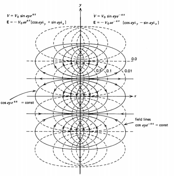
we write the solution separately for positive and negative x as

\[V = \left \{ \begin{matrix} V_{0} \sin ay \: e^{-ax}, & x \geq 0 \\ V_{0} \sin ay \: e^{ax}, & x \leq 0 \end{matrix} \right. \]

where we picked the amplitude coefficients to be continuous and match the excitation at x = 0. The electric field is then

\[\textbf{E} = - \nabla V = \left \{ \begin{matrix} -V_{0}a \: e^{-ax} [ \cos \: ay \textbf{i}_{y} - \sin \: ay \textbf{i}_{x}], & x>0 \\ -V_{0}a \: e^{ax} [ \cos \: ay \textbf{i}_{y} + \sin \: ay \textbf{i}_{x}], & x<0 \end{matrix} \right. \]

The surface charge density on the sheet is given by the discontinuity in normal component of D across the sheet:

\[\sigma_{f}(x=0) = \varepsilon [ E_{x} (x = 0_{+}) - E_{x} (x = 0_{-})] \\ 2 \varepsilon V_{0} a \: \sin \: ay \]

The field lines drawn in Figure 4-4 obey the equation

\[\frac{dy}{dx} = \frac{E_{y}}{E_{x}} = \mp \cot \: ay \Rightarrow \cos \: ay e^{mp ax} = \textrm{const} \left \{ \begin{matrix} x>0 \\ x<0 \end{matrix} \right. \]

4-2-5 Rectangular Harmonics

When excitations are not sinusoidally periodic in space, they can be made so by expressing them in terms of a trigonometric Fourier series. Any periodic function of y can be expressed as an infinite sum of sinusoidal terms as

\[f(y) = \frac{1}{2} b_{0} + \sum_{n=1}^{\infty} \bigg(a_{n} \: \sin \frac{2n \pi y}{\lambda} + b_{n} \cos \frac{2n \pi y}{\lambda} \bigg) \]

where \(\lambda\) is the fundamental period of f(y).

The Fourier coefficients a_n are obtained by multiplying both sides of the equation by sin (\(2 p \pi y/\lambda\) ) and integrating over a period. Since the parameter p is independent of the index n, we may bring the term inside the summation on the right hand side. Because the trigonometric functions are orthogonal to one another, they integrate to zero except when the function multiplies itself:

\[\int_{0}^{\lambda} \sin \frac{2 p \pi y}{\lambda} \sin \frac{2n \pi y}{\lambda} dy = \left \{ \begin{matrix} 0, & p \neq n \\ \lambda/2, & p = n \end{matrix} \right. \\ \int_{0}^{\lambda} \sin \frac{2 p \pi y}{\lambda} \cos \frac{2 n \pi y}{\lambda} dy = 0 \]

Every term in the series for \(n \neq p\) integrates to zero. Only the term for n = p is nonzero so that

\[a_{p} = \frac{2}{\lambda} \int_{0}^{\lambda} f(y) \sin \frac{2 p \pi y}{\lambda} dy \]

To obtain the coefficients b_n, we similarly multiply by cos (\(2 p \pi y/\lambda\)) and integrate over a period:

\[b_{p} = \frac{2}{\lambda} \int_{0}^{\lambda} f(y) \cos \frac{2 p \pi y}{\lambda} dy \]

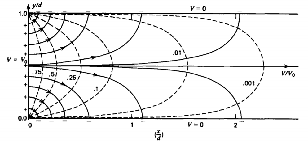
Consider the conducting rectangular box of infinite extent in the x and z directions and of width d in the y direction shown in Figure 4-5. The potential along the x = 0 edge is V_o while all other surfaces are grounded at zero potential. Any periodic function can be used for f(y) if over the interval \(0 \leq y \leq d, f(y)\) has the properties

\[f(y) = V_{0}, 0< y< d; f(y=0) = f(y=d) =0 \]

Figure 4-5 An open conducting box of infinite extent in the x and z directions and of finite width d in the y direction, has zero potential on all surfaces except the closed end at x = 0, where V = V₀.

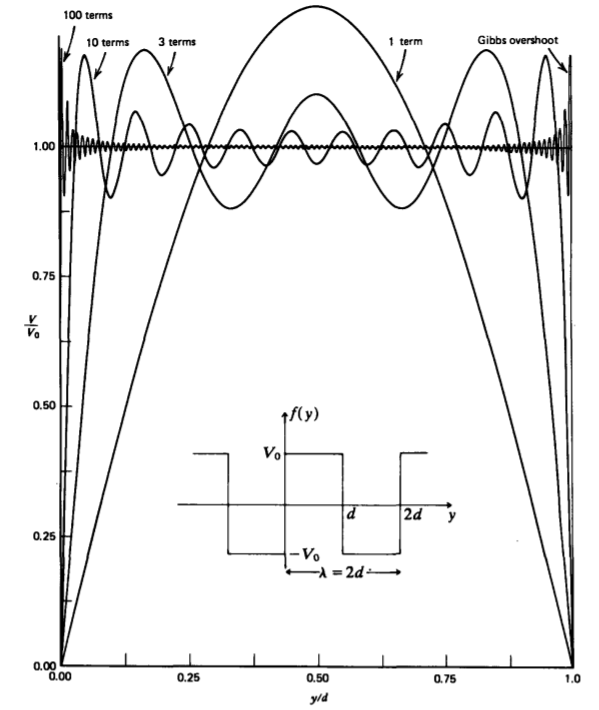
In particular, we choose the periodic square wave function with \(\lambda = 2d\) shown in Figure 4-6 so that performing the integrations in (28) and (29) yields

\[a_{p} = - \frac{2 V_{0}}{p \pi} (\cos p \pi - 1) \\ = \left \{ \begin{matrix} 0, & p \textrm{ even} \\ 4 V_{0}/p \pi, & p \textrm{ odd} \end{matrix} \right. \\ b_{p} = 0 \]

Thus the constant potential at x =0 can be written as the Fourier sine series

\[V(x=0) = V_{0} = \frac{4 V_{0}}{\pi} \sum_{n=1 \\ n \textrm{ odd}}^{\infty} \frac{\sin (n \pi y/d)}{n} \]

In Figure 4-6 we plot various partial sums of the Fourier series to show that as the number of terms taken becomes large, the series approaches the constant value V₀ except for the Gibbs overshoot of about 18% at y = 0 and y = d where the function is discontinuous.

The advantage in writing V₀ in a Fourier sine series is that each term in the series has a similar solution as found in (22) where the separation constant for each term is \(k_{n} =n \pi /d\) with associated amplitude \(4 V_{0} /(n \pi)\).

The solution is only nonzero for x > 0 so we immediately write down the total potential solution as

\[V(x,y) = \frac{4V_{0}}{\pi} \sum_{n=1 \\ n \textrm{ odd}}^{\infty} \frac{1}{n} \sin \frac{n pi y}{d} e^{-n \pi x /d} \]

Figure 4-5 for various partial sums. As the number of terms increases, the series approaches a constant except at the boundaries where the discontinuity in potential gives rise to the Gibbs phenomenon of an 18% overshoot with narrow width.

The electric field is then

\[\textbf{E} = - \nabla V = - \frac{4 V_{0}}{d} \sum_{n=1 \\ n \textrm{ odd}}^{\infty} \bigg( - \sin \frac{n \pi y}{d} \textbf{i}_{x} + \cos \frac{n \pi y}{d} \textbf{i}_{y} \bigg) e^{-n \pi x/d} \]

The field and equipotential lines are sketched in Figure 4-5. Note that for x>> d, the solution is dominated by the first harmonic. Far from a source, Laplacian solutions are insensitive to the details of the source geometry.

4-2-6 Three-Dimensional Solutions

If the potential depends on the three coordinates (x, y, z), we generalize our approach by trying a product solution of the form

\[V(x, y, z) = X (x) Y (y) Z (z) \]

which, when substituted into Laplace's equation, yields after division through by XYZ

\[\frac{1}{X} \frac{d^{2}X}{dx^{2}} + \frac{1}{Y} \frac{d^{2}Y}{dy^{2}} + \frac{1}{Z} \frac{d^{2}Z}{dz^{2}} = 0 \]

three terms each wholly a function of a single coordinate so that each term again must separately equal a constant:

\[\frac{1}{X} \frac{d^{2}X}{dx^{2}} = - k^{2}_{x}, \: \: \: \: \frac{1}{Y} \frac{d^{2}Y}{dy^{2}} = -k^{2}_{y}, \: \: \: \: \frac{1}{Z} \frac{d^{2}Z}{dz^{2}} = k_{x}^{2} + k_{y}^{2} \]

We change the sign of the separation constant for the z dependence as the sum of separation constants must be zero. The solutions for nonzero separation constants are

\[ \begin{array}{l}
X=A_1 \sin k_x x+A_2 \cos k_x x \\
Y=B_1 \sin k_y y+B_2 \cos k_y y \\
Z=C_1 \sinh k_z z+C_2 \cosh k_z z=D_1 e^{k_z z}+D_2 e^{-k_z z}
\end{array} \]

The solutions are written as if k_x, k_y, and k_z are real so that the x and y dependence is trigonometric while the z dependence is hyperbolic or equivalently exponential. However, k_x, k_y, or k_z may be imaginary converting hyperbolic functions to trigonometric and vice versa. Because the squares of the separation constants must sum to zero at least one of the solutions in (38) must be trigonometric and one must be hyperbolic. The remaining solution may be either trigonometric or hyperbolic depending on the boundary conditions. If the separation constants are all zero, in addition to the solutions of (6) we have the similar addition

\[Z = e_{1}z + f_{1} \]