4.3: Separation of Variables in Cylindrical Geometry

Product solutions to Laplace's equation in cylindrical coordinates

\[\frac{1}{\textrm{r}} \frac{\partial}{\partial \textrm{r}} \bigg( \textrm{r} \frac{\partial V}{\partial r} \bigg) + \frac{1}{\textrm{r}^{2}} \frac{\partial^{2}V}{\partial \phi^{2}} + \frac{\partial^{2}V}{dz^{2}} = 0 \]

also separate into solvable ordinary differential equations.

4-3-1 Polar Solutions

If the system geometry does not vary with z, we try a solution that is a product of functions which only depend on the radius r and angle \(\phi\):

\[V (\textrm{r,} \phi) = \textrm{R}(\textrm{r}) \Phi (\phi) \]

which when substituted into (1) yields

\[\frac{\Phi}{\textrm{r}} \frac{d}{d \textrm{r}} \bigg( \textrm{r} \frac{d \textrm{R}}{d \textrm{r}} \bigg) + \frac{\textrm{R}}{\textrm{r}^{2}} \frac{d^{2} \Phi}{d \phi^{2}} = 0 \]

This assumed solution is convenient when boundaries lay at a constant angle of \(\phi\) or have a constant radius, as one of the functions in (2) is then constant along the boundary.

For (3) to separate, each term must only be a function of a single variable, so we multiply through by r²/R \(\Phi\) and set each term equal to a constant, which we write as n ²:

\[\frac{\textrm{r}}{\textrm{R}} \frac{d}{d \textrm{r}} \bigg( \textrm{r} \frac{d \textrm{R}}{d \textrm{r}} \bigg) = n^{2}, \: \: \: \: \frac{1}{\Phi} \frac{d^{2} \Phi}{d \phi^{2}} = - n^{2} \]

The solution for \(\Phi\) is easily solved as

\[\Phi = \left \{ \begin{matrix} A_{1} \sin n \phi + A_{2} \cos n \phi, & n \neq 0 \\ B_{1} \phi + B_{2}, & n = 0 \end{matrix} \right. \]

The solution for the radial dependence is not as obvious. However, if we can find two independent solutions by any means, including guessing, the total solution is uniquely given as a linear combination of the two solutions. So, let us try a power-law solution of the form

\[\textrm{R} = A \textrm{r}^{p} \]

which when substituted into (4) yields

\[p^{2} = n^{2} \Rightarrow p = \pm n \]

For \(n \neq 0\), (7) gives us two independent solutions. When n =0 we refer back to (4) to solve

\[\textrm{r} \frac{d \textrm{R}}{d \textrm{r}} = \textrm{const} \Rightarrow \textrm{R} = D_{1} \ln \textrm{r} + D_{2} \]

so that the solutions are

\[\textrm{R} = \left \{ \begin{matrix} C_{1} \textrm{r}^{n} + C_{2} \textrm{r}^{-n}, & n \neq 0 \\ D_{1} \ln \textrm{r} + D_{2}, & n=0 \end{matrix} \right. \]

We recognize the n =0 solution for the radial dependence as the potential due to a line charge. The n =0 solution for the \(\phi\) dependence shows that the potential increases linearly with angle. Generally, n can be any complex number, although in usual situations where the domain is periodic and extends over the whole range \(0 \leq \phi \leq 2 \pi\), the potential at \(\phi = 2 \pi\) must equal that at \(\phi\) = 0 since they are the same point. This requires that n be an integer.

Example 4.3.1

Two planes of infinite extent in the z direction at an angle a to one another, as shown in Figure 4-7, are at a potential difference v. The planes do not intersect but come sufficiently close to one another that fringing fields at the electrode ends may be neglected. The electrodes extend from r = a to r = b. What is the approximate capacitance per unit length of the structure?

Figure 4-7 Two conducting planes at angle \(\alpha\) stressed by a voltage v have a \(\phi\)-directed electric field.

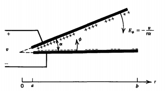
Solution

We try the n =0 solution of (5) with no radial dependence as

\(V = B_{1} \phi + B_{2}\)

The boundary conditions impose the constraints

\(V(\phi = 0) = 0, \: \: \: \: V(\phi = \alpha) = v \Rightarrow V = v \phi / \alpha\)

The electric field is

\(E_{\phi} = - \frac{1}{\textrm{r}} \frac{dV}{d \phi} = - \frac{v}{\textrm{r} \alpha} \)

The surface charge density on the upper electrode is then

\(\sigma_{f} (\phi = \alpha) = - \varepsilon E_{\phi} (\phi = \alpha) = \frac{\varepsilon v}{\textrm{r} \alpha}\)

with total charge per unit length

\(\lambda (\phi = \alpha) = \int_{\textrm{r} =a}^{b} \sigma_{f} (\phi = \alpha) d \textrm{r} = \frac{\varepsilon v}{\alpha} \ln \frac{b}{a}\)

so that the capacitance per unit length is

\(C = \frac{\lambda}{v} = \frac{\varepsilon \: \ln (b/a)}{\alpha}\)

4-3-2 Cylinder in a Uniform Electric Field

(a) Field Solutions

An infinitely long cylinder of radius a, permittivity \(\varepsilon_{2}\), and Ohmic conductivity \(\sigma_{2}\) is placed within an infinite medium of permittivity \(\varepsilon_{1}\) and conductivity \(\sigma_{1}\). A uniform electric field at infinity \(\textbf{E} = E_{0} \textbf{i}_{x}\), is suddenly turned on at t =0. This problem is analogous to the series lossy capacitor treated in Section 3-6-3. As there, we will similarly find that:

(i) At t = 0 the solution is the same as for two lossless dielectrics, independent of the conductivities, with no interfacial surface charge, described by the boundary condition

\[\sigma_{f} (\textrm{r} = a) = D_{\textrm{r}} (\textrm{r} = a_{+}) - D_{\textrm{r}}(\textrm{r} = a_{-}) = 0 \\ \Rightarrow \varepsilon_{1} E_{\textrm{r}}(\textrm{r} = a_{+}) = \varepsilon_{2}E_{\textrm{r}}(\textrm{r} = a_{-}) \]

(ii) As \(t \rightarrow \infty\), the steady-state solution depends only on the conductivities, with continuity of normal current at the cylinder interface,

\[J_{\textrm{r}}(\textrm{r} = a_{+}) = J_{\textrm{r}}(\textrm{r} = a_{-}) \Rightarrow \sigma_{1} E_{\textrm{r}}(\textrm{r} = a_{+}) = \sigma_{2} E_{\textrm{r}}(\textrm{r} = a_{-}) \]

(iii) The time constant describing the transition from the initial to steady-state solutions will depend on some weighted average of the ratio of permittivities to conductivities.

To solve the general transient problem we must find the potential both inside and outside the cylinder, joining the solutions in each region via the boundary conditions at r = a.

Trying the nonzero n solutions of (5) and (9), n must be an integer as the potential at \(\phi = 0\) and \(\phi = 2 \pi\) must be equal, since they are the same point. For the most general case, an infinite series of terms is necessary, superposing solutions with n = 1, 2, 3, 4, ... . However, because of the form of the uniform electric field applied at infinity, expressed in cylindrical coordinates as

\[\textbf{E} (\textrm{r} \rightarrow \infty) = E_{0} \textbf{i}_{x} = E_{0}[\textbf{i}_{\textrm{r}} \cos \phi - \textbf{i}_{\phi} \sin \phi] \]

we can meet all the boundary conditions using only the n = 1 solution.

Keeping the solution finite at r =0, we try solutions of the form

\[V(\textrm{r}, \phi) = \left \{ \begin{matrix} A(t) \textrm{r} \cos \phi, & \textrm{r} \leq a \\ [B(t) \textrm{r} + C(t)/ \textrm{r}] \cos \phi, & r \geq a \end{matrix} \right. \]

with associated electric field

\[\textbf{E} = - \nabla V = \left \{ \begin{matrix} -A (t) [ \cos \phi \textbf{i}_{r} - \sin \phi \textbf{i}_{\phi}] = - A(t) \textbf{i}_{x}, & \textrm{r} < \textrm{a} \\ - [\textbf{B}(t) - C(t)/ \textrm{r}^{2}] \cos \phi \textbf{i}_{\textrm{r}} \\ + [B(t) + C(t)/ \textrm{r}^{2}] \sin \phi \textbf{i}_{\phi}, & \textrm{r} > \textrm{a} \end{matrix} \right. \]

We do not consider the sin \(\phi\) solution of (5) in (13) because at infinity the electric field would have to be y directed:

\[V = D \textrm{r} \sin \phi \Rightarrow \textbf{E} = - \nabla V = - D [ \textbf{i}_{\textrm{r}} \sin \phi + \textbf{i}_{\phi} \cos \phi ] = -D \textbf{i}_{y} \]

The electric field within the cylinder is x directed. The solution outside is in part due to the imposed x-directed uniform field, so that as r \(\rightarrow \infty\) the field of (14) must approach (12), requiring that \(B(t) = E_{0}\). The remaining contribution to the external field is equivalent to a two-dimensional line dipole (see Problem 3.1), with dipole moment per unit length:

\[p_{x} = \lambda d = 2 \pi \varepsilon C (t) \]

The other time-dependent amplitudes A (t) and C(t) are found from the following additional boundary conditions:

(i) the potential is continuous at r= a, which is the same as requiring continuity of the tangential component of E:

\[V(\textrm{r} = a_{+}) = V(\textrm{r} = a_{-}) \Rightarrow E_{\phi}(\textrm{r} = a_{-}) = E_{\phi} (\textrm{r} = a_{+}) \\ \Rightarrow Aa = Ba + C/a \]

(ii) charge must be conserved on the interface

\[J_{\textrm{r}} (\textrm{r} = a_{+}) - J_{\textrm{r}}(\textrm{r} = a_{-}) + \frac{\partial \sigma_{f}}{\partial t} = - \\ \Rightarrow \sigma_{1} E_{\textrm{r}} (\textrm{r} = a_{+}) - \sigma_{2} E_{\textrm{r}}(\textrm{r} = a_{-}) \\ + \frac{\partial}{\partial t} [ \varepsilon_{1} E_{\textrm{r}}(\textrm{r} = a_{+}) - \varepsilon_{2} E_{\textrm{r}}(\textrm{r} = a_{-})]= 0 \]

In the steady state, (18) reduces to (11) for the continuity of normal current, while for t =0 the time derivative must be noninfinite so \(\sigma_{f}\) is continuous and thus zero as given by (10).

Using (17) in (18) we obtain a single equation in C(t):

\[\frac{dC}{dt} + \bigg( \frac{\sigma_{1} + \sigma_{2}}{\varepsilon_{1} + \varepsilon_{2}}\bigg) C = \frac{-a^{2}}{\varepsilon_{1} + \varepsilon_{2}} \bigg( E_{0} (\sigma_{1} - \sigma_{2}) + ( \varepsilon_{1} - \varepsilon_{2}) \frac{dE_{0}}{dt} \bigg) \]

Since \(E_{0}\) is a step function in time, the last term on the right-hand side is an impulse function, which imposes the initial condition

\[C(t=0) = -a^{2} \frac{(\varepsilon_{1} - \varepsilon_{2})}{\varepsilon_{1} + \varepsilon_{2}}E_{0} \]

so that the total solution to (19) is

\[C(t) = a^{2}E_{0} \bigg( \frac{\sigma_{1} - \sigma_{2}}{\sigma_{1} + \sigma_{2}} + \frac{2 (\sigma_{1} \varepsilon_{2} - \sigma_{2} \varepsilon_{1})}{(\sigma_{1} + \sigma_{2}) (\varepsilon_{1} + \varepsilon_{2})} e^{-t/\tau}\bigg), \: \: \: \tau = \frac{\varepsilon_{1} + \varepsilon_{2}}{\sigma_{1} + \sigma_{2}} \]

The interfacial surface charge is

\[\sigma_{f} (\textrm{r} = \textrm{a}, t) = \varepsilon_{1} E_{\textrm{r}}(\textrm{r} = \textrm{a}_{+}) - \varepsilon_{2} E_{\textrm{r}}(\textrm{r} = a_{-}) \\ = \bigg[ - \varepsilon_{1} \bigg( B = \frac{C}{a^{2}}\bigg) + \varepsilon_{2}A \bigg] \cos \phi \\ = \bigg[ (\varepsilon_{1} = \varepsilon_{2}) E_{0} + (\varepsilon_{1} + \varepsilon_{2}) \frac{C}{a^{2}} \bigg] \cos \phi \\ = \frac{2 (\sigma_{2} \varepsilon_{1} - \sigma_{1} \varepsilon_{2})}{\sigma_{1} + \sigma_{2}} E_{0}[1 - e^{-t/\tau}] \cos \phi \]

The upper part of the cylinder (\(- \pi/2 \leq \phi \leq \pi/2) is charged of one sign while the lower half (\(\pi/2 \leq \phi \leq \frac{3}{2} \pi\)) is charged with the opposite sign, the net charge on the cylinder being zero. The cylinder is uncharged at each point on its surface if the relaxation times in each medium are the same, \(\varepsilon_{1}/\sigma_{1} = \varepsilon_{2}/\sigma_{2}\)

The solution for the electric field at t =0 is

\[\textbf{E} (t = 0) = \left \{ \begin{matrix} \frac{2 \varepsilon_{1} E_{0}}{\varepsilon_{1} + \varepsilon_{2}} [\cos \phi \textbf{i}_{\textrm{r}} - \sin \phi \textbf{i}_{\phi}] = \frac{2 \varepsilon_{1} E_{0}}{\varepsilon_{1} + \varepsilon_{2}} \textbf{i}_{x}, & \textrm{r} < a\\ E_{0} \bigg[ \bigg( 1 + \frac{a^{2}}{\textrm{r}^{2}} \frac{\varepsilon_{2} - \varepsilon_{1}}{\varepsilon_{1} + \varepsilon_{2}} \bigg) \cos \phi \textbf{i}_{\textrm{r}} \\ - \bigg(1 - \frac{a^{2}}{\textrm{r}^{2}} \frac{\varepsilon_{2} - \varepsilon_{1}}{\varepsilon_{1} + \varepsilon_{2}} \bigg) \sin \phi \textbf{i}_{\phi} \bigg], & \textrm{r} >a \end{matrix} \right. \]

The field inside the cylinder is in the same direction as the applied field, and is reduced in amplitude if \(\varepsilon_{2} > \varepsilon_{1}\) and increased in amplitude if \(\varepsilon_{2} < \varepsilon_{1}\), up to a limiting factor of two as \(\varepsilon_{1}\) becomes large compared to \(\varepsilon_{2}\). If \(\varepsilon_{2} - \varepsilon_{1}\), the solution reduces to the uniform applied field everywhere.

The dc steady-state solution is identical in form to (23) if we replace the permittivities in each region by their conductivities;

\[ \mathbf{E}(t \rightarrow \infty)=\left\{\begin{array}{cc}
\frac{2 \sigma_1 E_0}{\sigma_1+\sigma_2}\left[\cos \phi \mathbf{i}_{\mathrm{r}}-\sin \phi \mathbf{i}_\phi\right]=\frac{2 \sigma_1 E_0}{\sigma_1+\sigma_2} \mathbf{i}_{\mathrm{x}}, & \mathrm{r}<a \\
E_0\left[\left(1+\frac{a^2}{\mathrm{r}^2} \frac{\sigma_2-\sigma_1}{\sigma_1+\sigma_2}\right) \cos \phi \mathbf{i}_{\mathrm{r}}\right. & \\
\left.-\left(1-\frac{a^2}{\mathrm{r}^2} \frac{\sigma_2-\sigma_1}{\sigma_1+\sigma_2}\right) \sin \phi \mathbf{i}_\phi\right], & \mathrm{r}>a
\end{array}\right. \]

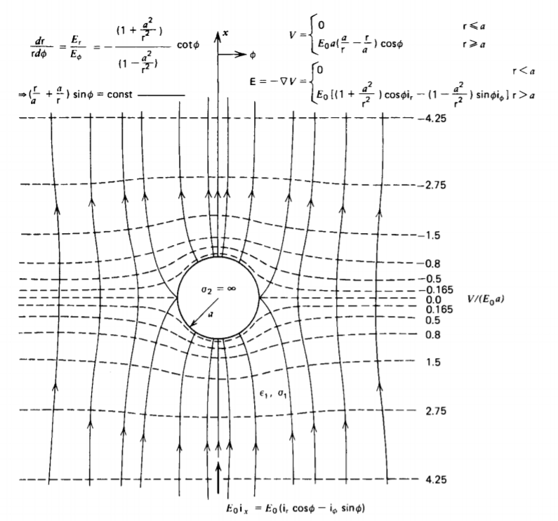
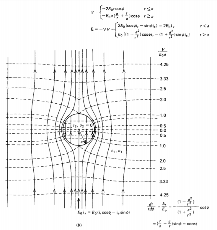
(b) Field Line Plotting

Because the region outside the cylinder is charge free, we know that \(\nabla \cdot \textbf{E} = 0 \). From the identity derived in Section 1-5-4b, that the divergence of the curl of a vector is zero, we thus know that the polar electric field with no z component can be expressed in the form

\[\textbf{E} (\textrm{r}, \phi) = \nabla \times \Sigma (\textrm{r}, \phi) \textbf{i}_{z} \\ = \frac{1}{\textrm{r}} \frac{\partial \Sigma}{\partial \phi} \textbf{i}_{\textrm{r}} - \frac{\partial \Sigma}{\partial \textrm{r}} \textbf{i}_{\phi} \]

where \(\Sigma\) is called the stream function. Note that the stream function vector is in the direction perpendicular to the electric field so that its curl has components in the same direction as the field.

Along a field line, which is always perpendicular to the equipotential lines,

\[\frac{d \textrm{r}}{\textrm{r} d \phi} = \frac{E_{\textrm{r}}}{E_{\phi}} = - \frac{1}{\textrm{r}} \frac{\partial \Sigma /\partial \phi}{\partial \Sigma/ \partial \textrm{r}} \]

By cross multiplying and grouping terms on one side of the equation, (26) reduces to

\[d \Sigma = \frac{\partial \Sigma}{\partial \textrm{r}}d \textrm{r} + \frac{\partial \Sigma}{\partial \phi} d \phi = 0 \Rightarrow \sigma = \textrm{const} \]

Field lines are thus lines of constant \(\Sigma\).

For the steady-state solution of (24), outside the cylinder

\[ \begin{array}{l}
\frac{1}{\mathrm{r}} \frac{\partial \Sigma}{\partial \phi}=E_{\mathrm{r}}=E_0\left(1+\frac{a^2}{\mathrm{r}^2} \frac{\sigma_2-\sigma_1}{\sigma_1+\sigma_2}\right) \cos \phi \\
-\frac{\partial \Sigma}{\partial \mathrm{r}}=E_\phi=-E_0\left(1-\frac{a^2}{\mathrm{r}^2} \frac{\sigma_2-\sigma_1}{\sigma_1+\sigma_2}\right) \sin \phi
\end{array} \]

we find by integration that

\[\sigma = E_{0} \bigg( \textrm{r} + \frac{a^{2}}{\textrm{r}} \frac{\sigma_{2} - \sigma_{1}}{\sigma_{1} + \sigma_{2}} \bigg) \sin \phi \]

The steady-state'field and equipotential lines are drawn in Figure 4-8 when the cylinder is perfectly conducting (\(\sigma_{2} \rightarrow x \)) or perfectly insulating (\(\sigma_{2}\) = 0).

If the cylinder is highly conducting, the internal electric field is zero with the external electric field incident radially, as drawn in Figure 4-8a. In contrast, when the cylinder is perfectly insulating, the external field lines must be purely tangential to the cylinder as the incident normal current is zero, and the internal electric field has double the strength of the applied field, as drawn in Figure 4-8b.

4-3-3 Three-Dimensional Solutions

If the electric potential depends on all three coordinates, we try a product solution of the form

\[V( \textrm{r}, \phi , z) = \textrm{R}(\textrm{r}) \Phi (\phi) Z (z) \]

which when substituted into Laplace's equation yields

\[\frac{Z \Phi}{\textrm{r}} \frac{d}{d \textrm{r}} \bigg( \textrm{r} \frac{d \textrm{R}}{d \textrm{r}} + \frac{\textrm{R} Z}{\textrm^{2}} \frac{d^{2} \Phi}{d \phi^{2}} + \textrm{R} \Phi \frac{d^{2} Z}{d z^{2}} = 0 \]

We now have a difficulty, as we cannot divide through by a factor to make each term a function only of a single variable.

Figure 4-8 Steady-state field and equipotential lines about a (a) perfectly conducting or (b) perfectly insulating cylinder in a uniform electric field.

However, by dividing through by \(V = \textrm{R} \Phi Z\)

\[ \underbrace{\frac{1}{\operatorname{Rr}} \frac{d}{d \mathrm{r}}\left(\mathrm{r} \frac{d \mathrm{R}}{d \mathrm{r}}\right)+\frac{1}{\mathrm{r}^2 \Phi} \frac{d^2 \Phi}{d \phi^2}}_{-k^2}+\underbrace{\frac{1}{Z} \frac{d^2 Z}{d z^2}}_{k^2}=0 \]

we see that the first two terms are functions of r and \(\phi\) while the last term is only a function of z. This last term must therefore equal a constant:

\[\frac{1}{Z} \frac{d^{2}Z}{dz^{2}} = k^{2} \Rightarrow Z = \left \{ \begin{matrix} A_{1} \sinh kz + A_{2} \cosh kz, & k \neq 0 \\ A_{3}z + A_{4}, & k = 0 \end{matrix} \right. \]

Figure 4-8b

The first two terms in (32) must now sum to -k² so that after multiplying through by r² we have

\[ \frac{\mathrm{r}}{\mathrm{R}} \frac{d}{d \mathrm{r}}\left(\mathrm{r} \frac{d \mathrm{R}}{d \mathrm{r}}\right)+k^2 \mathrm{r}^2+\frac{1}{\Phi} \frac{d^2 \Phi}{d \phi^2}=0  \]

Now again the first two terms are only a function of r, while the last term is only a function of \(\phi\) so that (34) again separates:

\[\frac{\textrm{r}}{\textrm{R}} \frac{d}{d \textrm{r}} \bigg( \textrm{r} \frac{d \textrm{R}}{d \textrm{r}} \bigg) + k^{2} \textrm{r}^{2} = n^{2}, \: \: \: \: \frac{1}{\Phi} \frac{d^{2} \Phi}{d \phi^{2}} = - n^{2} \]

\[
\Phi=\left\{\begin{array}{ll}
B_1 \sin n \phi+B_2 \cos n \phi, & n \neq 0 \\
B_3 \phi+B_4, & n=0
\end{array}\right.
\]
The resulting differential equation for the radial dependence
\[
\mathrm{r} \frac{d}{d \mathrm{r}}\left(\mathrm{r} \frac{d \mathrm{R}}{d \mathrm{r}}\right)+\left(k^2 \mathrm{r}^2-n^2\right) \mathrm{R}=0
\]
is Bessel's equation and for nonzero \(k\) has solutions in terms of tabulated functions:

\[\textrm{R} = \left \{ \begin{matrix} C_{1}J_{n}(k \textrm{r}) + C_{2} Y_{n}(k \textrm{r}, & k \neq 0 \\ C_{3}\textrm{r}^{n} + C_{4} \textrm{r}^{-n}, & k = 0, \: \: \: \: n \neq 0 \\ C_{5} \ln \textrm{r} + C_{6}, & k= 0, \: \: \: \: n = 0 \end{matrix} \right. \]

where J_n is called a Bessel function of the first kind of order n and Y_n is called the nth-order Bessel function of the second kind. When n = 0, the Bessel functions are of zero order while if k =0 the solutions reduce to the two-dimensional solutions of (9).

Some of the properties and limiting values of the Bessel functions are illustrated in Figure 4-9. Remember that k

Figure 4-9b

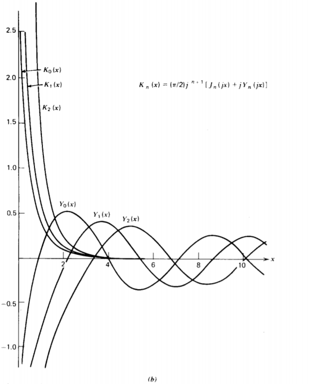
can also be purely imaginary as well as real. When k is real so that the z dependence is hyperbolic or equivalently exponential, the Bessel functions are oscillatory while if k is imaginary so that the axial dependence on z is trigonometric, it is convenient to define the nonoscillatory modified Bessel functions as

\[I_{n} (k \textrm{r} ) = j^{-n} J_{n}(jk \textrm{r}) \\ K_{n}(k \textrm{r}) = \frac{\pi}{2} j^{n + 1} [J_{n}(jk \textrm{r}) + j Y_{n} )jk \textrm{r})] \]

As in rectangular coordinates, if the solution to Laplace's equation decays in one direction, it is oscillatory in the perpendicular direction.

4-3-4 High Voltage Insulator Bushing

The high voltage insulator shown in Figure 4-10 consists of a cylindrical disk with Ohmic conductivity \(\sigma\) supported by a perfectly conducting cylindrical post above a ground plane.*

The plane at z = 0 and the post at r = a are at zero potential, while a constant potential is imposed along the circumference of the disk at r = b. The region below the disk is free space so that no current can cross the surfaces at z = L and z = L - d. Because the boundaries lie along surfaces at constant z or constant r we try the simple zero separation constant solutions in (33) and (38), which are independent of angle \(\phi\):

\[V(\textrm{r}, z) = \left \{ \begin{matrix} A_{1}z = D_{1}z \: \ln \: \textrm{r} + C_{1} \: \ln \textrm{r} + D_{1}, & L - D < z < L \\ A_{2}z + B_{2} z \: \ln \: \textrm{r} + C_{2} \: \ln \: \textrm{r} + D_{2}, & 0 \leq z \leq L -d \end{matrix} \right. \]

Applying the boundary conditions we relate the coefficients as

\[V(z=0) = 0 \Rightarrow C_{2} = D_{2} = 0 \\ V(\textrm{r} = a) = 0 \Rightarrow \left \{ \begin{matrix} A_{2} + B_{2} \ln \: a = 0 \\ A_{1} + B_{2} \ln \: a = 0 \\ C_{1} \ln \: a + D_{1} = 0 \end{matrix} \right. \\ V(\textrm{r} = b, z > L - d) = V_{0} \Rightarrow \left \{ \begin{matrix} A_{1} + B_{1} \ln \: b = 0 \\ C_{1} \ln \: b + D_{1} = V_{0} \end{matrix} \right. \\ V(z = (L-d)_{-}) = V(z = (L-d)_{+}) \Rightarrow (L-d) (A_{2} + B_{2} \ln \: \textrm{r} ) \\ = (L-d)(A_{1} + B_{1} \ln \: \textrm{r}) + C_{1} \ln \: \textrm{r} + D_{1} \]

Figure 4-10 (a) A finitely conducting disk is mounted upon a perfectly conducting cylindrical post and is placed on a perfectly conducting ground plane. (b) Field and equipotential lines

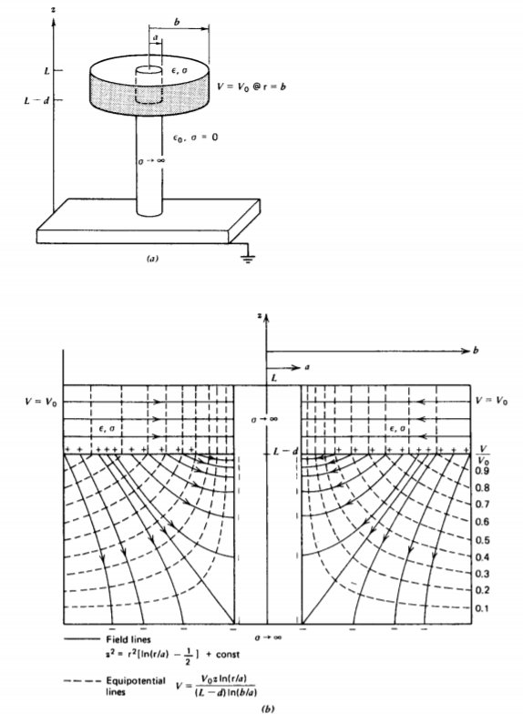
which yields the values

\[A_{1} = B_{1} = 0, \: \: \: \: C_{1} = \frac{V_{0}}{\ln (b/a)}, \: \: \: \: D_{1} = - \frac{V_{0} \ln a}{\ln (b/a)} \\ A_{2} = - \frac{V_{0} \ln a}{(L-d) \ln (b/a)}, \: \: \: \: B_{2} = \frac{V_{0}}{(L-d) \ln (b/a)}, \: \: \: \: C_{2} = D_{2} = 0 \]

The potential of (40) is then
\[
V(\mathrm{r}, z)=\left\{\begin{array}{ll}
\frac{V_0 \ln (\mathrm{r} / a)}{\ln (b / a)}, & L-d \leq z \leq L \\
\frac{V_0 z \ln (\mathrm{r} / a)}{(L-d) \ln (b / a)}, & 0 \leq z \leq L-d
\end{array}\right.
\]
with associated electric field
\[
\mathbf{E}=-\nabla V=\left\{\begin{array}{ll}
-\frac{V_0}{\mathrm{r} \ln (b / a)} \mathbf{i}_{\mathrm{r}}, & L-d<z<L \\
-\frac{V_0}{(L-d) \ln (b / a)}\left(\ln \frac{\mathrm{r}}{a} \mathbf{i}_z+\frac{z}{\mathbf{i}_{\mathbf{r}}}\right), & 0<z<L-d
\end{array}\right.
\]

The field lines in the free space region are

\[\frac{d \textrm{r}}{dz} = \frac{E_{\textrm{r}}}{E_{z}} = \frac{z}{\textrm{r} \ln (\textrm{r}/a)} \Rightarrow z^{2} = \textrm{r}^{2} \bigg[ \ln \frac{\textrm{r}}{a} - \frac{1}{2} \bigg] + \textrm{const} \]

and are plotted with the equipotential lines in Figure 4-10b.

* M. N. Horenstein, "Particle Contamination of High Voltage DC Insulators," PhD thesis, Massachusetts Institute of Technology, 1978.