4.4: Product Solutions in Spherical Geometry

In spherical coordinates, Laplace's equation is

\[\frac{1}{r^{2}} \frac{\partial}{\partial r} \bigg( r^{2} \frac{\partial V}{\partial r} \bigg) + \frac{1}{r^{2} \sin^{2} \theta} \frac{\partial^{2}V}{\partial \phi^{2}} = 0 \]

4-4-1 One-Dimensional Solutions

If the solution only depends on a single spatial coordinate, the governing equations and solutions for each of the three coordinates are

(i)

\[\frac{d}{dr} \bigg( r^{2} \frac{dV(r)}{dr} \bigg) = 0 \Rightarrow V(r) = \frac{A_{1}}{r} + A_{2} \]

(ii)

\[ \frac{d}{d \theta} \bigg( \sin \theta \frac{dV(\theta)}{d \theta} \bigg) = 0 \Rightarrow V(\theta) = B_{1} \ln \bigg( \tan \frac{\theta}{2} \bigg) + B_{2} \]

(iii)

\[\frac{d^{2} V(\phi)}{d \phi^{2}} = 0 \Rightarrow V (\phi) = C_{1} \phi + C_{2} \]

We recognize the radially dependent solution as the potential due to a point charge. The new solutions are those which only depend on \(\theta\) or \(\phi\).

Example 4-2: Two Cones

Two identical cones with surfaces at angles \(\theta = \alpha\) and \(\theta = \pi - \alpha\) and with vertices meeting at the origin, are at a potential difference v, as shown in Figure 4-11. Find the potential and electric field.

Figure 4-11 Two cones with vertices meeting at the origin are at a potential difference v.

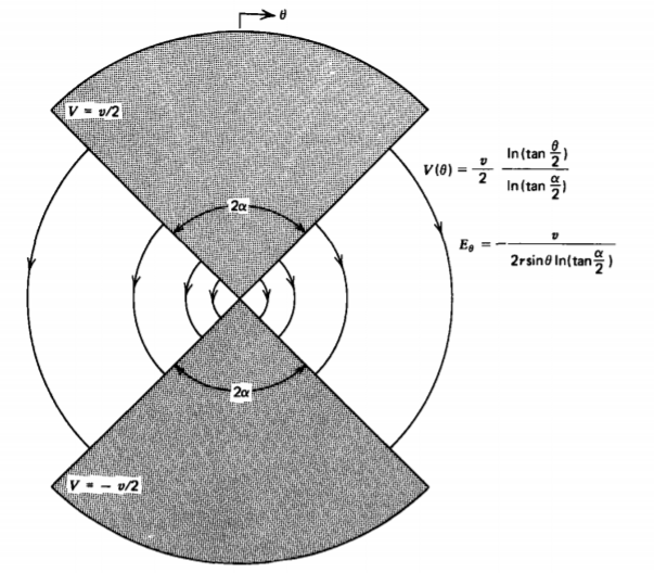
Solution

Because the boundaries are at constant values of \(\theta\), we try (3) as a solution:

\(V (\theta) = B_{1} \ln [ \tan (\theta/2)] + B_{2} \nonumber \)

From the boundary conditions we have

\(V(\theta = \alpha) = \frac{v}{2} \\ V(\theta = \pi - \alpha) = \frac{-v}{2} \Rightarrow B_{1} = \frac{v}{2 \ln [ \tan(\alpha/2)]}, \: \: \: \: B_{2} = 0  \nonumber \)

so that the potential is

\[V(\theta) = \frac{v}{2} \frac{\ln [ \tan (\theta/2)]}{\ln [ \tan (\alpha/2)]} \nonumber \]

with electric field

\[\textbf{E} = - \nabla V = \frac{-v}{2r \: \sin \theta \ln [ \tan (\alpha /2)]} \textbf{i}_{\theta} \nonumber \]

4-4-2 Axisymmetric Solutions

If the solution has no dependence on the coordinate \(\phi\), we try a product solution

\[V(r, \theta) = R(r) \Theta (\theta) \]

which when substituted into (1), after multiplying through by \(r^{2}/R \Theta\), yields

\[\frac{1}{R} \frac{d}{dr} \bigg( r^{2} \frac{dR}{dr} \bigg) + \frac{1}{\Theta \sin \theta} \frac{d}{d \theta} \bigg( \sin \theta \frac{d \Theta}{d \theta} \bigg) = 0 \]

Because each term is again only a function of a single variable, each term is equal to a constant. Anticipating the form of the solution, we choose the separation constant as n(n + 1) so that (6) separates to

\[ \frac{d}{dr} \bigg( r^{2} \frac{dR}{dr} \bigg) - n (n+1) R = 0 \]

\[ \frac{d}{d \theta} \bigg( \sin \theta \frac{d \Theta}{d \theta} \bigg) + n (n + 1) \Theta \sin \theta = 0 \]

For the radial dependence we try a power-law solution

\[R = A r^{p} \]

which when substituted back into (7) requires

\[p(p + 1) = n (n + 1) \]

which has the two solutions

\[p = n, \: \: \: \: p = -(n+1) \]

When n = 0 we re-obtain the 1/r dependence due to a point charge.

To solve (8) for the \(\theta\) dependence it is convenient to introduce the change of variable

\[\beta = \cos \theta \]

so that

\[\frac{d \Theta}{d \theta} = \frac{d \Theta}{d \beta} \frac{d \beta}{d \theta} = - \sin \theta \frac{d \Theta}{d \beta} = - (1 - \beta^{2})^{1/2} \frac{d \Theta}{d \beta} \]

Then (8) becomes

\[\frac{d}{d \beta} \bigg( (1-\beta^{2}) \frac{d \Theta}{d \beta} \bigg) + n (n + 1) \Theta = 0 \]

which is known as Legendre's equation. When n is an integer, the solutions are written in terms of new functions:

\[\Theta = B_{n} P_{n} (\beta) + C_{n} Q_{n} (\beta) \]

where the \(P_{n} (\beta)\) are called Legendre polynomials of the first kind and are tabulated in Table 4-1. The Q_n solutions are called the Legendre functions of the second kind for which the first few are also tabulated in Table 4-1. Since all the Q_n are singular at \(\theta = 0\) and \(\theta = \pi\), where \(\beta = \pm 1\), for all problems which include these values of angle, the coefficients C_n in (15) must be zero, so that many problems only involve the Legendre polynomials of first kind, \(P_{n}( \cos \theta)\). Then using (9)-(11) and (15) in (5), the general solution for the potential with no \(\phi\) dependence can be written as

\[V(r, \theta) = \sum_{n=0}^{\infty} (A_{n}r^{n} + B_{n}r^{-(n+1)}) P_{n}(\cos \theta) \]

Table 4-1 Legendre polynomials of first and second kind

n	\( P_{n}(\beta = \cos \theta)\)	\(Q_{n}(\beta = \cos \theta)\)
0	1	\(\frac{1}{2} \ln \bigg( \frac{1 + \beta}{1 - \beta} \bigg)\)
1	\(\beta = \cos \theta\)	\(\frac{1}{2} \beta \ln \bigg( \frac{1 + \beta}{1 - \beta} \bigg) - 1\)
2	\(\frac{1}{2}(3 \beta^{2} - 1) = \frac{1}{2} (3 \cos^{2} \theta =1)\)	\(\frac{1}{4}(3 \beta^{2}-1) \ln \bigg( \frac{1 + \beta}{1 - \beta}\bigg) - \frac{3 \beta}{2}\)
3	\(\frac{1}{2}(5 \beta^{3} - 3 \beta) = \frac{1}{2}(5 \cos^{3} \theta - 3 \cos \theta)\)	\(\frac{1}{4}(5 \beta^{3} - 3 \beta) \ln \bigg( \frac{1 + \beta}{1 - \beta} \bigg) - \frac{5}{2} \beta^{2} + \frac{2}{3}\)
...
m	\(\frac{1}{2^{m}m!} \frac{d^{m}}{d \beta^{m}}(\beta^{2} - 1)^{m}\)

4-4-3 Conducting Sphere in a Uniform Field

(a) Field Solution

A sphere of radius R, permittivity \(\varepsilon_{2}\), and Ohmic conductivity \(\sigma_{2}\) is placed within a medium of permittivity \(\varepsilon_{1}\) and conductivity \(\sigma_{1}\). A uniform dc electric field \(E_{0} \textbf{i}_{x}\) is applied at infinity. Although the general solution of (16) requires an infinite number of terms, the form of the uniform field at infinity in spherical coordinates,

\[\textbf{E}(r \rightarrow \infty) = E_{0} \textbf{i}_{z} = E_{0}(\textbf{i}_{r} \cos \theta - \textbf{i}_{\theta} \sin \theta ) \]

suggests that all the boundary conditions can be met with just the n = 1 solution:

\[V(r, \theta) = \left \{ \begin{matrix} Ar \: \cos \theta, & r \leq R \\ (Br + C/r^{2}) \cos \theta, & r \geq R \end{matrix} \right. \]

We do not include the \(1/r^{2}\) solution within the sphere (r< R) as the potential must remain finite at r =0. The associated electric field is

\[\textbf{E} = - \nabla V = \left \{ \begin{matrix} - A (\textbf{i}_{r} \cos \theta - \textbf{i}_{\theta} \sin \theta) = -A \textbf{i}_{z}, & r<R \\ -(B- 2 C/r^{3}) \cos \theta \textbf{i}_{r} + (B + C/r^{3}) \sin \theta \textbf{i}_{\theta}, & r > R \end{matrix} \right. \]

The electric field within the sphere is uniform and z directed while the solution outside is composed of the uniform z-directed field, for as \(r \rightarrow \infty\) the field must approach (17) so that \(B = -E_{0}\), plus the field due to a point dipole at the origin, with dipole moment

\[p_{z} = 4 \pi \varepsilon_{1}C \]

Additional steady-state boundary conditions are the continuity of the potential at r= R [equivalent to continuity of tangential E(r =R)], and continuity of normal current at r= R,

\[V(r=R_{+}) = V(r = R_{-}) \Rightarrow E_{\theta} (r = R_{+}) = E_{\theta}(r = R_{-}) \\ \Rightarrow AR = BR + CR^{2} \\ J_{r} (r = R_{+}) = J_{r}(r = R_{-}) \Rightarrow \sigma_{1} E_{r} (r = R_{+}) = \sigma_{2} E_{r} (r = R_{-}) \\ \Rightarrow \sigma_{1}(B - 2 C/R^{3}) = \sigma_{2}A \]

for which solutions are

\[A = - \frac{3 \sigma_{1}}{2 \sigma_{1} + \sigma_{2}} E_{0}, \: \: \: \: B = - E_{0}, \: \: \: \: C = \frac{(\sigma_{2} - \sigma_{1})R^{3}}{2 \sigma_{1} + \sigma_{2}} E_{0} \]

The electric field of (19) is then

\[\textbf{E} = \left \{ \begin{matrix} \frac{3 \sigma_{1} E_{0}}{2 \sigma_{1} + \sigma_{2}} (\textbf{i}_{r} \cos \theta - \textbf{i}_{\theta} \sin \theta) = \frac{3 \sigma_{1} E_{0}}{2 \sigma_{1} + \sigma_{2}} \textbf{i}_{z}, & r <R \\ E_{0} \bigg[ \bigg( 1 + \frac{2 R^{3} (\sigma_{2} - \sigma_{1})}{r^{3} (2 \sigma_{1} + \sigma_{2})} \bigg) \cos \theta \textbf{i}_{r} \\ - \bigg( 1 - \frac{R^{3} (\sigma_{2} - \sigma_{1})}{r^{3}(2 \sigma_{1} + \sigma_{2})} \bigg) \sin \theta \textbf{i}_{\theta} \bigg], & r > R \end{matrix} \right. \]

The interfacial surface charge is

\[\sigma_{f} (r = R) = \varepsilon_{1} E_{r} (r = R_{+}) - \varepsilon_{2} E_{r} (r = R_{-}) \\ = \frac{3 (\sigma_{2} \varepsilon_{1} - \sigma_{1} \varepsilon_{2}) E_{0}}{2 \sigma_{1} + \sigma_{2}} \cos \theta \]

which is of one sign on the upper part of the sphere and of opposite sign on the lower half of the sphere. The total charge on the entire sphere is zero. The charge is zero at every point on the sphere if the relaxation times in each region are equal:

\[\frac{\varepsilon_{1}}{\sigma_{1}} = \frac{\varepsilon_{2}}{\sigma_{2}} \]

The solution if both regions were lossless dielectrics with no interfacial surface charge, is similar in form to (23) if we replace the conductivities by their respective permittivities.

(b) Field Line Plotting

As we saw in Section 4-3-2b for a cylindrical geometry, the electric field in a volume charge-free region has no divergence, so that it can be expressed as the curl of a vector. For an axisymmetric field in spherical coordinates we write the electric field as

\[\textbf{E}(r, \theta) = \nabla \times \bigg( \frac{\Sigma (r, \theta)}{r \sin \theta} \textbf{i}_{\phi} \bigg) \\ = \frac{1}{r^{2} \sin \theta} \frac{\partial \Sigma}{\partial \theta} \textbf{i}_{r} - \frac{1}{r \sin \theta} \frac{\partial \Sigma}{\partial r} \textbf{i}_{\theta} \]

Note again, that for a two-dimensional electric field, the stream function vector points in the direction orthogonal to both field components so that its curl has components in the same direction as the field. The stream function \(\Sigma\) is divided by \(r \sin \theta\) so that the partial derivatives in (26) only operate on \(\Sigma\).

The field lines are tangent to the electric field

\[\frac{dr}{r d \theta} = \frac{E_{r}}{E_{\theta}} = - \frac{1}{r} \frac{\partial \Sigma/ \partial \theta}{\partial \Sigma/ \partial r} \]

which after cross multiplication yields

\[d \Sigma = \frac{\partial \Sigma}{\partial r} + \frac{\partial \Sigma}{\partial \theta} = 0 \Rightarrow \Sigma = \textrm{const} \]

so that again \(\Sigma\) is constant along a field line.

For the solution of (23) outside the sphere, we relate the field components to the stream function using (26) as

\[E_{r} = \frac{1}{r^{2} \sin \theta} \frac{\partial \Sigma}{\partial \theta} = E_{0} \bigg(1 + \frac{2R^{3}(\sigma_{2} - \sigma_{1})}{r^{3}(2 \sigma_{1} + \sigma_{2})} \bigg) \cos \theta \\ E_{\theta} = - \frac{1}{r \sin \theta} \frac{\partial \Sigma}{\partial r} = - E_{0} \bigg( 1 - \frac{R^{3}(\sigma_{2} - \sigma_{1})}{r^{3}(2 \sigma_{1} + \sigma_{2})} \bigg) \sin \theta \]

so that by integration the stream function is

\[\Sigma = E_{0} \bigg( \frac{r^{2}}{2} + \frac{R^{3} (\sigma_{2} - \sigma_{1})}{r (2 \sigma_{1} + \sigma_{2})} \bigg) \sin^{2} \theta \]

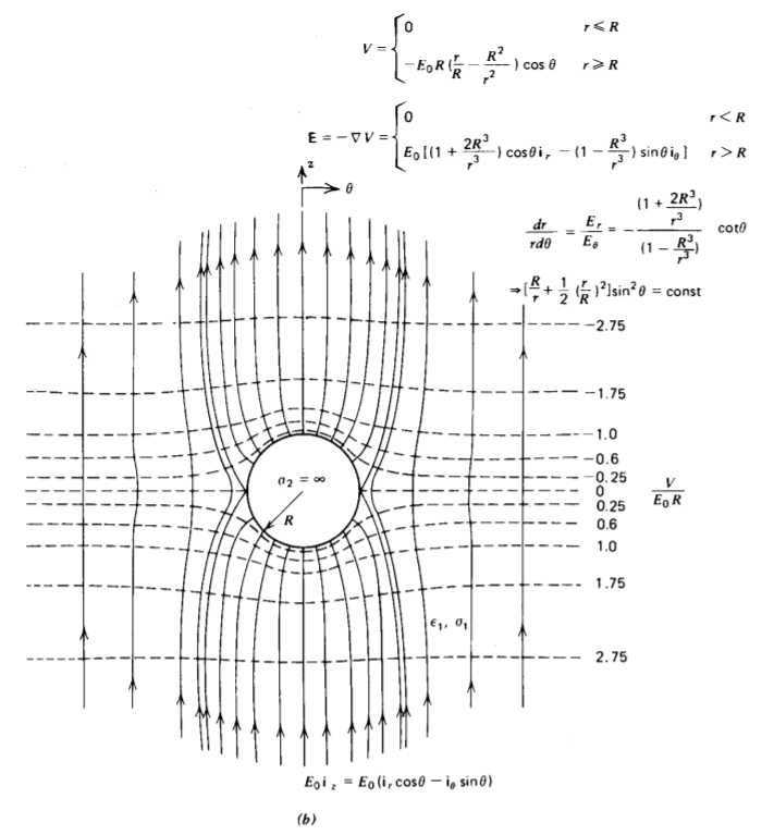
The steady-state field and equipotential lines are drawn in Figure 4-12 when the sphere is perfectly insulating (Or \(\sigma_{2} = 0\)) or perfectly conducting (\(\sigma_{2} \rightarrow \infty\)).

Figure 4-12 Steady-state field and equipotential lines about a (a) perfectly insulating or (b) perfectly conducting sphere in a uniform electric field.

Figure 4-12b

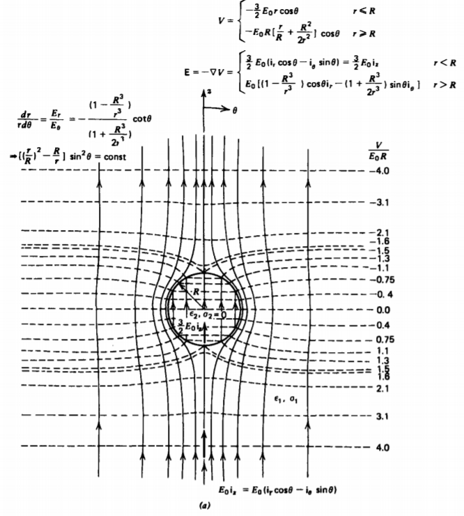
If the conductivity of the sphere is less than that of the surrounding medium (\(\sigma_{2} < \sigma_{1}\)) the electric field within the sphere is larger than the applied field. The opposite is true for (\(\sigma_{2} > \sigma_{1}\)). For the insulating sphere in Figure 4-12a, the field lines go around the sphere as no current can pass through.

For the conducting sphere in Figure 4-12b, the electric field lines must be incident perpendicularly. This case is used as a polarization model, for as we see from (23) with \(\sigma_{2} \rightarrow \infty\), the external field is the imposed field plus the field of a point dipole with moment,

\[p_{z} = 4 \pi \varepsilon_{1} R^{3} E_{0} \]

If a dielectric is modeled as a dilute suspension of noninteracting, perfectly conducting spheres in free space with number density N, the dielectric constant is

\[\varepsilon = \frac{\varepsilon_{0} E_{0} + P}{E_{0}} = \frac{\varepsilon_{0} E_{0} + N p_{z}}{E_{0}} = \varepsilon_{0}(1 + 4 \pi R^{3} N) \]

4-4-4 Charged Particle Precipitation Onto a Sphere

The solution for a perfectly conducting sphere surrounded by free space in a uniform electric field has been used as a model for the charging of rain drops.* This same model has also been applied to a new type of electrostatic precipitator where small charged particulates are collected on larger spheres.**

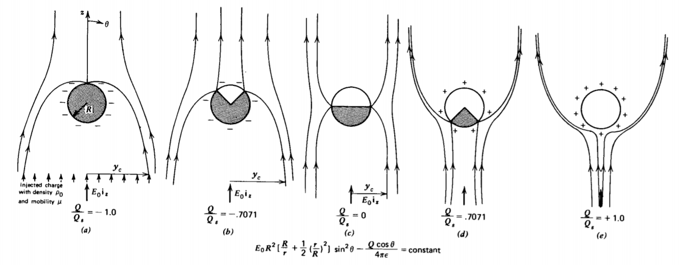
Then, in addition to the uniform field \(E_{0}\textbf{i}_{z}\) applied at infinity, a uniform flux of charged particulate with charge density \(\rho_{0}\), which we take to be positive, is also injected, which travels along the field lines with mobility \(\mu\). Those field lines that start at infinity where the charge is injected and that approach the sphere with negative radial electric field, deposit charged particulate, as in Figure 4-13. The charge then redistributes itself uniformly on the equipotential surface so that the total charge on the sphere increases with time. Those field lines that do not intersect the sphere or those that start on the sphere do not deposit any charge.

We assume that the self-field due to the injected charge is very much less than the applied field \(E_{0}\). Then the solution of (23) with \(\sigma_{2} = \infty\) is correct here, with the addition of the radial field of a uniformly charged sphere with total charge Q(t):

\[\textbf{E} + \bigg[ E_{0} \bigg(1 + \frac{2R^{3}}{r^{3}} \bigg) \cos \theta + \frac{Q}{4 \pi \varepsilon r^{2}} \bigg] \textbf{i}_{r} - E_{0} \bigg( 1 - \frac{R^{3}}{r^{3}} \bigg) \sin \theta \textbf{i}_{\theta}, \: \: \: \: r > R \]

Charge only impacts the sphere where E_r(r=R) is negative:

\[ E_r(r=R)=3 E_0 \cos \theta+\frac{Q}{4 \pi \varepsilon R^2}<0 \]

Figure 4-13 Electric field lines around a uniformly charged perfectly conducting sphere in a uniform electric field with continuous positive charge injection from \(z = - \infty\). Only those field lines that impact on the sphere with the electric field radially inward [E_r (R) <0] deposit charge. (a) If the total charge on the sphere starts out as negative charge with magnitude greater or equal to the critical charge, the field lines within the distance y_c of the z axis impact over the entire sphere. (b)-(d) As the sphere charges up it tends to repel some of the incident charge and only part of the sphere collects charge. With increasing charge the angular window for charge collection decreases as does y_c. (e) For \(Q \geq Q\), no further charge collects on the sphere so that the charge remains constant thereafter. The angular window and y_c have shrunk to zero.

which gives us a window for charge collection over the range of angle, where

\[\cos \theta \leq - \frac{Q}{12 \pi \varepsilon E_{0} R^{2}} \]

Since the magnitude of the cosine must be less than unity, the maximum amount of charge that can be collected on the sphere is

\[Q_{s} = 12 \pi \varepsilon E_{0} R^{2} \]

As soon as this saturation charge is reached, all field lines emanate radially outward from the sphere so that no more charge can be collected. We define the critical angle \(\theta_{c}\) as the angle where the radial electric field is zero, defined when (35) is an equality \(\cos \theta_{c} = -Q/Q_{s}\). The current density charging the sphere is

\[J_{r} = \rho_{0} \mu E_{r} (r = R) \\ = 3 \rho_{0} \mu E_{0} (\cos \theta + Q/Q_{s}), \: \: \: \: \: \theta_{c} < \theta < \pi \]

The total charging current is then

\[\frac{dQ}{dt} = - \int_{\theta = \theta_{c}}^{\pi} J_{r} 2 \pi R^{2} \sin \theta d \theta \\ = - 6 \pi \rho_{0} \mu E_{0} R^{2} \int_{\theta = \theta_{c}}^{\pi} (\cos \theta + Q/Q_{s} \) \sin \theta d \theta \\ = -6 \pi \rho_{0} \mu E_{0} R^{2} ( - \frac{1}{4} \cos 2 \theta - (Q/Q_{s}) \cos \theta) \vert_{\theta = \theta_{c}}^{\pi} = - 6 \pi \rho_{0} \mu E_{0} R^{2} ( - \frac{1}{4} ( 1- \cos 2 \theta_{c}) + (Q/Q_{s}) ( 1 + \cos theta_{c})) \]

As long as \(\vert Q \vert < Q_{s}, \: \: \: \theta_{c}\) is define by the equality in (35). If Q exceeds Q_s, which can only occur if the sphere is intentionally overcharged, then \(\theta_{c} = \pi\) and no further charging can occur as \(dQ/dt\) in (38) is zero. If Q is negative and exceeds Q_s in magnitude, \(Q < -Q_{s}\), then the whole sphere collects charge as \(\theta_{c} = 0\). Then for these conditions we have

\[\cos \theta_{c} = \left \{ \begin{matrix} -1, & Q>Q_{s} \\ -Q/Q_{s} & -Q_{s} < Q < Q_{s} \\ 1, & Q< - Q_{s} \end{matrix} \right. \]

\[\cos 2 \theta_{c} = 2 \cos^{2} \theta_{c} - 1 = \left \{ \begin{matrix} 1, & \vert Q \vert > Q_{s} \\ 2 (Q/Q_{s})^{2} - 1, & \vert Q \vert < Q_{s} \end{matrix} \right. \]

so that (38) becomes

\[\frac{d \frac{Q}{Q_{s}}}{dt} = \left \{ \begin{matrix} 0, & Q>Q_{s} \\ \frac{\rho_{0} \mu}{4 \varepsilon} \bigg(1 - \frac{Q}{Q_{s}} \bigg)^{2}, & -Q_{s} < Q < Q_{s} \\ - \frac{\rho_{0}\mu}{\varepsilon} \frac{Q}{Q_{s}}, & Q < - Q_{s} \end{matrix} \right. \]

with integrated solutions

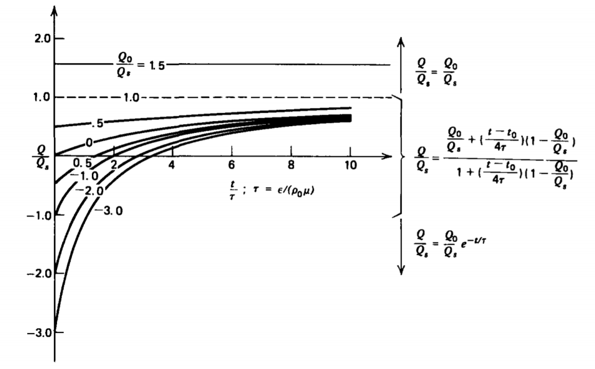
\[\frac{Q}{Q_{s}} = \left \{ \begin{matrix} \frac{Q_{0}}{Q_{s}}, & Q > Q_{s} \\ \frac{\frac{Q_{0}}{Q_{s}} + \frac{(t - t_{0})}{4 \tau} \bigg(1 - \frac{Q_{0}}{Q_{s}}\bigg)}{1 + \frac{(t-t_{0})}{4 \tau} \bigg(1 = - \frac{Q_{0}}{Q_{s}} \bigg)}, & -Q_{s} < Q < Q_{s} \\ \frac{Q_{0}}{Q_{s}} e^{-t/Tau}, & Q< -Q_{s} \end{matrix} \right. \]

where Q_o is the initial charge at t=0 and the characteristic charging time is

\[\tau = \varepsilon/ (\rho_{0} \mu) \]

If the initial charge Q₀ is less than -Q_s, the charge magnitude decreases with the exponential law in (42) until the total charge reaches -Q_s at t = t₀. Then the charging law switches to the next regime with \(Q_{0} = - Q_{s}\), where the charge passes through zero and asymptotically slowly approaches \(Q = Q_{s}\). The charge can never exceed Q_s unless externally charged. It then remains constant at this value repelling any additional charge. If the initial charge Q₀ has magnitude less than Q_s, then \(t_{0} = 0 \). The time dependence of the charge is plotted in Figure 4-14 for various initial charge values Q₀. No matter the initial value of \(Q_{0}\) for \(Q < Q_{s}\), it takes many time constants for the charge to closely approach the saturation value Q_s. The force of repulsion on the injected charge increases as the charge on the sphere increases so that the charging current decreases.

The field lines sketched in Figure 4-13 show how the fields change as the sphere charges up. The window for charge collection decreases with increasing charge. The field lines are found by adding the stream function of a uniformly charged sphere with total charge Q to the solution of (30)

Figure 4-14 There are three regimes describing the charge build-up on the sphere. It takes many time constants ( \(\tau = \varepsilon/\rho_{0}/mu) \)  for the charge to approach the saturation value Q_s because as the sphere charges up the Coulombic repulsive force increases so that most of the charge goes around the sphere. If the sphere is externally charged to a value in excess of the saturation charge, it remains constant as all additional charge is completely repelled.

with \(\sigma_{2} \rightarrow \infty\)

\[\Sigma = E_{0}R^{2} \bigg[ \frac{R}{r} + \frac{1}{2} \bigg( \frac{r}{R} \bigg) ^{2} \bigg] \sin^{2} \theta - \frac{Q \cos \theta}{4 \pi \varepsilon} \]

The streamline intersecting the sphere at r = R, \(\theta = \theta_{c}\) separates those streamlines that deposit charge onto the sphere from those that travel past.

* See: F. J. W. Whipple and J. A. Chalmers, On Wilson's Theory of the Collection of Charge by Falling Drops, Quart. J. Roy. Met. Soc. 70, (1944), p. 103.

** See: H. J. White, Industrial Electrostatic Precipitation Addison-Wesley, Reading. Mass. 1963, pp. 126-137.