4.5: A Successive Method - Numerical Relaxation

In many cases, the geometry and boundary conditions are irregular so that closed form solutions are not possible. It then becomes necessary to solve Poisson's equation by a computational procedure. In this section we limit ourselves to dependence on only two Cartesian coordinates.

4-5-1 Finite Difference Expansions

The Taylor series expansion to second order of the potential V, at points a distance \(\Delta_{x}\) on either side of the coordinate (x, y), is

\[V(x + \Delta x, y) \approx V(x,y) + \frac{\partial V}{\partial x} \bigg|_{x, y} \: \Delta x + \frac{1}{2} \frac{\partial^{2} V}{\partial x^{2}} \bigg|_{x,y} \: ( \Delta x)^{2} \\ V(x-\Delta x, y) \approx V (x,y) - \frac{\partial V}{\partial x} \bigg|_{x,y} \Delta x + \frac{1}{2} \frac{\partial^{2} V}{\partial x ^{2}} \bigg|_{x,y} \: (\Delta x)^{2} \]

If we add these two equations and solve for the second derivative, we have

\[\frac{\partial^{2}V}{\partial x^{2}} \approx \frac{V(x + \Delta x, y) + V(x-\Delta x, y) - 2 V (x,y)}{(\Delta x)^{2}} \]

Performing similar operations for small variations from y yields

\[\frac{\partial^{2}V}{\partial y^{2}} \approx \frac{V(x,y + \Delta y) + V(x,y - \Delta y) - 2 V (x,y)}{(\Delta y)^{2}} \]

If we add (2) and (3) and furthermore let \(\Delta x = \Delta y\), Poisson's equation can be approximated as

\[\frac{\partial^{2}V}{\partial x^{2}} + \frac{\partial^{2}V}{\partial y^{2}} \approx \frac{1}{(\Delta x)^{2}} [ V (x + \Delta x, y) + V(x - \Delta x, y) \\ + V(x,y + \Delta y) + V (x,y - \Delta y) - 4 V (x,y)] = - \frac{\partial_{f}(x,y)}{\varepsilon} \]

so that the potential at (x, y) is equal to the average potential of its four nearest neighbors plus a contribution due to any volume charge located at (x, y):

\[V(x,y) = \frac{1}{4} [V (x + \Delta x, y) + V(x- \Delta x, y) \\ + V (x,y + \Delta y) + V (x,y - \Delta y)] + \frac{\rho_{f} (x,y) (\Delta x)^{2}}{4 \varepsilon} \]

The components of the electric field are obtained by taking the difference of the two expressions in (1)

\[\begin{array}{l}
E_x(x, y)=-\left.\frac{\partial V}{\partial x}\right|_{x, y} \approx-\frac{1}{2 \Delta x}[V(x+\Delta x, y)-V(x-\Delta x, y)] \\
E_y(x, y)=-\left.\frac{\partial V}{\partial y}\right|_{x, y} \approx-\frac{1}{2 \Delta y}[V(x, y+\Delta y)-V(x, y-\Delta y)]
\end{array} \]

4-5-2 Potential Inside a Square Box

Consider the square conducting box whose sides are constrained to different potentials, as shown in Figure (4-15). We discretize the system by drawing a square grid with four

Figure 4-15 The potentials at the four interior points of a square conducting box with imposed potentials on its surfaces are found by successive numerical relaxation. The potential at any charge free interior grid point is equal to the average potential of the four adjacent points.

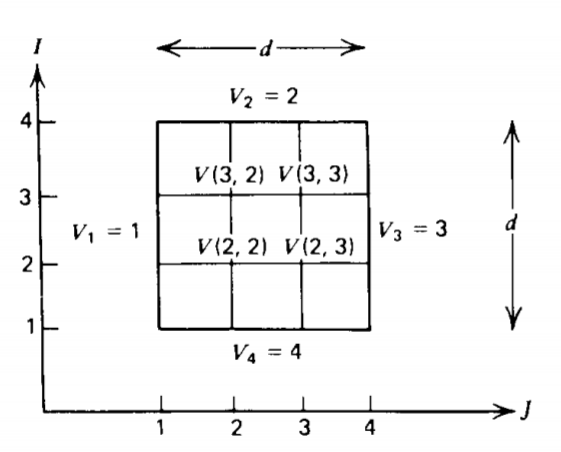
interior points. We must supply the potentials along the boundaries as proved in Section 4-1:

\[V_{1} = \sum_{I = 1}^{4} V (I, J = 1) =1, \: \: \: \: V_{3} = \sum_{I = 1}^{4} V (I, J = 4) = 3 \\ V_{2} = \sum_{J=1}^{4} V(I = 4, J) = 2, \: \: \: \: V_{4} = \sum_{J=1}^{4} V(I = 1, J) = 4 \]

Note the discontinuity in the potential at the corners.

We can write the charge-free discretized version of (5) as

\[V(I, J) = \frac{1}{4} [ V (I + 1, J ) + V(I-1, J) + V(I, J + 1) + V( I, J -1)] \]

We then guess any initial value of potential for all interior grid points not on the boundary. The boundary potentials must remain unchanged. Taking the interior points one at a time, we then improve our initial guess by computing the average potential of the four surrounding points.

We take our initial guess for all interior points to be zero inside the box:

\[V(2,2) = 0, \: \: \: \: V(3,3) = 0 \\ V(3,2) = 0, \: \: \: \: V(2, 3) = 0 \]

Then our first improved estimate for V(2, 2) is

\[V(2,2) = \frac{1}{4}[V (2,1) + V(2,3) + V(1,2) + V(3,2)] \\ \frac{1}{4} [1 + 0 + 4 + 0] = 1.25 \]

Using this value of V (2, 2) we improve our estimate for V (3, 2) as

\[V(3,2) = \frac{1}{4} [V (2,2) + V(4,2) + V (3,1) + V(3,3)] \\ \frac{1}{4}[1.25 + 2 + 1 + 0] = 1.0625 \]

Similarly for V(3, 3),

\[V(3,3) = \frac{1}{4}[V(3,2) + V(3,4) + V(2,3) + V(4,3)] \\ = \frac{1}{4}[ 1.0625 + 3 + 0 + 2] = 1.5156 \]

and V (2, 3)

\[V(2,3) = \frac{1}{4} [ V(2,2) + V(2,4) + V(1,3) + V(3,3)] \\ = \frac{1}{4}[1.25 + 3 + 4 + 1.5156] = 2.4414 \]

We then continue and repeat the procedure for the four interior points, always using the latest values of potential. As the number of iterations increase, the interior potential values approach the correct solutions. Table 4-2 shows the first ten iterations and should be compared to the exact solution to four decimal places, obtained by superposition of the rectangular harmonic solution in Section 4-2-5 (see problem 4-4):

\[V(x,y) = \sum_{n=1 \\ n \textrm{ odd}} ^{\infty} \frac{4}{n \pi \sinh n \pi} \bigg[ \sin \frac{n \pi y }{d} \bigg(V_{3} \sinh \frac{n \pi x}{d} - V_{1} \sinh \frac{n \pi(x-d)}{d} \bigg) \\ + \sin \frac{n \pi x}{d} \bigg(V_{2} \sinh \frac{n \pi y}{d} - V_{4} \sinh \frac{n \pi (y-d)}{d} \bigg) \bigg] \]

where V₁, V₂, V₃ and V₄ are the boundary potentials that for this case are

\[V_{1} = 1, \: \: \: V_{2} = 2, \: \: \: V_{3}=3, \: \: \: V_{4} = 4 \]

To four decimal places the numerical solutions remain unchanged for further iterations past ten.

Table 4-2 Potential values for the four interior points in Figure 4-15 obtained by successive relaxation for the first ten iterations

	0	1	2	3	4	5	6	7	8	9	10	Exact
V1	0	1.2500	2.1260	2.3777	2.4670	2.4911	2.4975	2.4993	2.4998	2.4999	2.5000	2.5000
V2	0	1.0625	1.6604	1.9133	1.9770	1.9935	1.9982	1.9995	1.9999	2.0000	2.0000	1.9771
V3	0	1.5156	2.2755	2.4409	2.4829	2.4952	2.4987	2.4996	2.4999	2.5000	2.5000	2.5000
V4	0	2.4414	2.8504	2.9546	2.9875	2.9966	2.9991	2.9997	2.9999	3.0000	3.0000	3.0229

The results are surprisingly good considering the coarse grid of only four interior points. This relaxation procedure can be used for any values of boundary potentials, for any number of interior grid points, and can be applied to other boundary shapes. The more points used, the greater the accuracy. The method is easily implemented as a computer algorithm to do the repetitive operations.