5.1: Forces on Moving Charges

5-1-1 The Lorentz Force Law

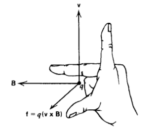
It was well known that magnets exert forces on each other, but in 1820 Oersted discovered that a magnet placed near a current carrying wire will align itself perpendicular to the wire. Each charge q in the wire, moving with velocity v in the magnetic field B [teslas, (kg-s^-2 -A^-1)], felt the empirically determined Lorentz force perpendicular to both v and B

\[\textbf{f} = q( \textbf{v} \times \textbf{B}) \]

as illustrated in Figure 5-1. A distribution of charge feels a differential force df on each moving incremental charge element dq:

\[d \textbf{f} = dq (\textbf{V} \times \textbf{B}) \]

Figure 5-1 A charge moving through a magnetic field experiences the Lorentz force perpendicular to both its motion and the magnetic field.

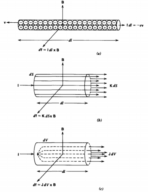
Moving charges over a line, surface, or volume, respectively constitute line, surface, and volume currents, as in Figure 5-2, where (2) becomes

\[d \textbf{f} = \left \{ \begin{matrix} \rho_{f} \textbf{v} \times \textbf{B} dV = \textbf{J} \times \textbf{B} dV & (\textbf{J} = \rho_{f} \textbf{v}, \: \textrm{ volume current density} ) \\ \sigma_{f} \textbf{v} \times \textbf{B} dS = \textbf{K} \times \textbf{B} dS & (\textbf{K} = \sigma_{f} \textbf{v}, \: \textrm{ surface current density}) \\ \lambda_{f} \textbf{v} \times \textbf{B} dl = \textbf{I} \times \textbf{B} dl & (\textbf{I} = \lambda_{f} \textbf{v}, \: \textrm{line current} ) \end{matrix} \right. \]

Figure 5-2 Moving line, surface, and volume charge distributions constitute currents. (a) In metallic wires the net charge is zero since there are equal amounts of negative and positive charges so that the Coulombic force is zero. Since the positive charge is essentially stationary, only the moving electrons contribute to the line current in the direction opposite to their motion. (b) Surface current. (c) Volume current.

The total magnetic force on a current distribution is then obtained by integrating (3) over the total volume, surface, or contour containing the current. If there is a net charge with its associated electric field E, the total force densities include the Coulombic contribution:

\[\textbf{f} = q (\textbf{E} + \textbf{v} \times \textbf{B}) \: \textrm{ Newton} \\ \textbf{F}_{L} = \lambda_{f} (\textbf{E} + \textbf{V} \times \textbf{B}) = \lambda_{f} \textbf{E} + \textbf{I} \times \textbf{B} \: \textrm{ N/m} \\ \textbf{F}_{S} = \sigma_{f} (\textbf{E} + \textbf{v} \times \textbf{B}) = \sigma_{f} \textbf{E} + \textbf{K} \times \textbf{B} \: \textrm{ N/m^{2}} \\ \textbf{F}_{V} = \rho_{f} (\textbf{E} + \textbf{v} \times \textbf{B}) = \rho_{f} \textbf{E} + \textbf{J} \times \textbf{B} \: \textrm{ N/m^{3}} \]

In many cases the net charge in a system is very small so that the Coulombic force is negligible. This is often true for conduction in metal wires. A net current still flows because of the difference in velocities of each charge carrier.

Unlike the electric field, the magnetic field cannot change the kinetic energy of a moving charge as the force is perpendicular to the velocity. It can alter the charge's trajectory but not its velocity magnitude.

5-1-2 Charge Motions in a Uniform Magnetic Field

The three components of Newton's law for a charge q of mass m moving through a uniform magnetic field \(B_{z} \textbf{i}_{z}\) are

\[m \frac{d \textbf{v}}{dt} = q \textbf{v} \times \textbf{B} \Rightarrow \left \{ \begin{matrix} m \frac{dv_{x}}{dt} = q v_{y} B_{z} \\ m \frac{dv_{y}}{dt} = - qv_{x}B_{z} \\ m \frac{dv_{z}}{dt} = 0 \Rightarrow v_{z} = \textrm{const} \end{matrix} \right. \]

The velocity component along the magnetic field is unaffected. Solving the first equation for \(v_{y}\) and substituting the result into the second equation gives us a single equation in \(v_{x}\):

\[\frac{d^{2}v_{x}}{dt^{2}} + \omega_{0}^{2}v_{x} = 0, \: \: \: \: v_{y} = \frac{1}{\omega_{0}} \frac{dv_{x}}{dt}, \: \: \: \: \omega_{0} = \frac{qB_{z}}{m} \]

where \(\omega_{0}\) is called the Larmor angular velocity or the cyclotron frequency (see Section 5-1-4). The solutions to (6) are

\[v_{x} = A_{1} \sin \omega_{0} t + A_{2} \cos \omega_{0} t \\ v_{y} = \frac{1}{\omega_{0}} \frac{dv_{x}}{dt} = A_{1} \cos \oemga_{0} t - A_{2} \sin \omega_{0} t \]

where \(A_{1}\) and \(A_{2}\) are found from initial conditions. If at t =0,

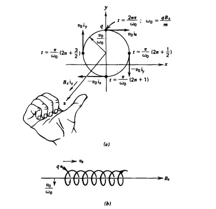
\[\textbf{v}(t = 0) = v_{0} \textbf{i}_{x} \]

then (7) and Figure 5-3a show that the particle travels in a circle, with constant speed \(v_{0}\) in the xy plane:

\[v = v_{0} (\cos \omega_{0} t \textbf{i}_{x} - \sin \omega_{0} t \textbf{i}_{y}) \]

with radius

\[R = v_{0}/\omega_{0} \]

If the particle also has a velocity component along the magnetic field in the z direction, the charge trajectory becomes a helix, as shown in Figure 5-3b.

Figure 5-3 (a) A positive charge q, initially moving perpendicular to a magnetic field, feels an orthogonal force putting the charge into a circular motion about the magnetic field where the Lorentz force is balanced by the centrifugal force. Note that the charge travels in the direction (in this case clockwise) so that its self-field through the loop [see Section 5-2-1] is opposite in direction to the applied field. (b) A velocity component in the direction of the magnetic field is unaffected resulting in a helical trajectory.

5-1-3 The Mass Spectrograph

The mass spectrograph uses the circular motion derived in Section 5-1-2 to determine the masses of ions and to measure the relative proportions of isotopes, as shown in Figure 5-4. Charges enter between parallel plate electrodes with a y directed velocity distribution. To pick out those charges with a particular magnitude of velocity, perpendicular electric and magnetic fields are imposed so that the net force on a charge is

\[f_{x} = q(E_{x} + v_{y}B_{z}) \]

For charges to pass through the narrow slit at the end of the channel, they must not be deflected by the fields so that the force in (11) is zero. For a selected velocity \(v_y=v_0\) this requires a negatively \(\boldsymbol{x}\) directed electric field
\[
E_x=\frac{V}{c}=-v_0 B_0
\]

which is adjusted by fixing the applied voltage V. Once the charge passes through the slit, it no longer feels the electric field and is only under the influence of the magnetic field. It thus travels in a circle of radius

\[r = \frac{v_{0}}{\omega_{0}} = \frac{v_{0}m}{q B_{0}} \]

Figure 5-4 The mass spectrograph measures the mass of an ion by the radius of its trajectory when moving perpendicular to a magnetic field. The crossed uniform electric field selects the ion velocity that can pass through the slit.

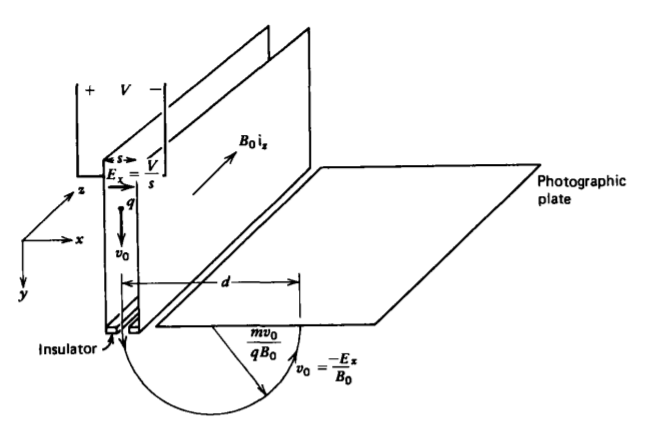
which is directly proportional to the mass of the ion. By measuring the position of the charge when it hits the photographic plate, the mass of the ion can be calculated. Different isotopes that have the same number of protons but different amounts of neutrons will hit the plate at different positions.

For example, if the mass spectrograph has an applied voltage of V= -100 V across a 1-cm gap (E_x = -10⁴ V/m) with a magnetic field of 1 tesla, only ions with velocity

\[v_{y} = - E_{x}/B_{0} = 10^{4} \textrm{m/sec} \]

will pass through. The three isotopes of magnesium, ₁₂Mg²⁴ , ₁₂Mg²⁵ , ₁₂Mg²⁶ , each deficient of one electron, will hit the photographic plate at respective positions:

\[d = 2r = \frac{2 \times 10^{4} N (1.67 \times 10^{-27})}{1.6 \times 10^{-19} (1)} \approx 2 \times 10^{-4} N \Rightarrow 0.48, 0.50, 0.52 \textrm{cm} \]

where N is the number of protons and neutrons (m = 1.67 x 10^-27 kg) in the nucleus.

5-1-4 The Cyclotron

A cyclotron brings charged particles to very high speeds by many small repeated accelerations. Basically it is composed of a split hollow cylinder, as shown in Figure 5-5, where each half is called a "dee" because their shape is similar to the

Figure 5-5 The cyclotron brings ions to high speed by many small repeated accelerations by the electric field in the gap between dees. Within the dees the electric field is negligible so that the ions move in increasingly larger circular orbits due to an applied magnetic field perpendicular to their motion.

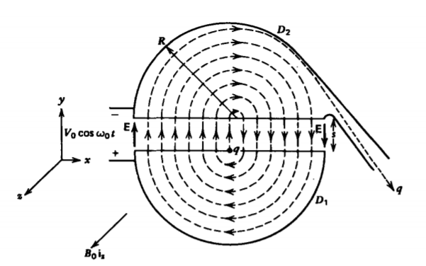
fourth letter of the alphabet. The dees are put at a sinusoidally varying potential difference. A uniform magnetic field \(B_{0} \textbf{i}_{z}\) is applied along the axis of the cylinder. The electric field is essentially zero within the cylindrical volume and assumed uniform \(E_{y} =v(t)/s\) in the small gap between dees. A charge source at the center of \(D_{1}\) emits a charge q of mass m with zero velocity at the peak of the applied voltage at t = 0. The electric field in the gap accelerates the charge towards D₂. Because the gap is so small the voltage remains approximately constant at V₀ while the charge is traveling between dees so that its displacement and velocity are

\[m \frac{dv_{y}}{dt} = \frac{qV_{0}}{\textrm{s}} \Rightarrow v_{y} = \frac{qV_{0}}{sm} t \\ v_{y} = \frac{dy}{dt} \Rightarrow y = \frac{qV_{0}t^{2}}{2 ms} \]

The charge thus enters D₂ at time \(t = [ 2ms^{2}/q \textrm{V}_{0}]^{1/2}\) later with velocity \(v_{y} = \sqrt{2qV_{0}/m}\). Within \(D_{2}\) the electric field is negligible so that the charge travels in a circular orbit of radius \(r = v_{y}/\omega_{0} = m v_{y} /q B_{0}\) due to the magnetic field alone. The frequency of the voltage is adjusted to just equal the angular velocity \(\omega_{0} = q B_{0}/m\) of the charge, so that when the charge re-enters the gap between dees the polarity has reversed accelerating- the charge towards D₁ with increased velocity. This process is continually repeated, since every time the charge enters the gap the voltage polarity accelerates the charge towards the opposite dee, resulting in a larger radius of travel. Each time the charge crosses the gap its velocity is increased by the same amount so that after n gap traversals its velocity and orbit radius are

\[v_{n} = \bigg( \frac{2qnV_{0}}{m} \bigg) ^{1/2}, \: \: \: \: R_{n} = \frac{v_{n}}{\omega_{0}} = \bigg( \frac{2 nm V_{0}}{qB_{0}^{2}} \bigg) ^{1/2} \]

If the outer radius of the dees is R, the maximum speed of the charge

\[ v_{\max }=\omega_0 R=\frac{q B_0}{m} R \]

is reached after \(2n = qB_{0}^{2}R^{2}/mV_{0}\) round trips when \(R_{n} = R\). For a hydrogen ion (\(q = 1.6 \times 10^{-19}\) coul, \(m = 1.67 \times 10^{-27}\) kg), within a magnetic field of 1 tesla (\(\omega_{0} \approx 9.6 \times 10^{7}\) radian/sec) and peak voltage of 100 volts with a cyclotron radius of one meter, we reach \(v_{\textrm{max}} = 9.6 \times 10^{7}\) m/s (which is about 30% of the speed of light) in about \(2n \approx 9.6 \times 10^{5}\) round-trips, which takes a time \( \tau = 4 n \pi/\omega_{0} \approx 2 \pi/100 \approx 0.06\) sec. To reach this

speed with an electrostatic accelerator would require

\[\frac{1}{2} mv^{2} = qV \Rightarrow V = \frac{mv^{2}_{\textrm{max}}}{2q} \approx 48 \times 10^{6} \textrm{Volts} \]

The cyclotron works at much lower voltages because the angular velocity of the ions remains constant for fixed \(qB_{0}/m\) and thus arrives at the gap in phase with the peak of the applied voltage so that it is sequentially accelerated towards the opposite dee. It is not used with electrons because their small mass allows them to reach relativistic velocities close to the speed of light, which then greatly increases their mass, decreasing their angular velocity \(\omega\), putting them out of phase with the voltage.

5-1-5 Hall Effect

When charges flow perpendicular to a magnetic field, the transverse displacement due to the Lorentz force can give rise to an electric field. The geometry in Figure 5-6 has a uniform magnetic field \(B_{0} \textbf{i}_{z}\) applied to a material carrying a current in the y direction. For positive charges as for holes in a p-type semiconductor, the charge velocity is also in the positive y direction, while for negative charges as occur in metals or in n-type semiconductors, the charge velocity is in the negative y direction. In the steady state where the charge velocity does not vary with time, the net force on the charges must be zero,

Figure 5-6 A magnetic field perpendicular to a current flow deflects the charges transversely giving rise to an electric field and the Hall voltage. The polarity of the voltage is the same as the sign of the charge carriers.

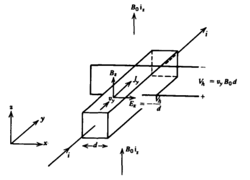
which requires the presence of an x-directed electric field

\[\textbf{E} + \textbf{v} \times \textbf{B} = 0 \Rightarrow E_{x} = - v_{y} B_{0} \]

A transverse potential difference then develops across the material called the Hall voltage:

\[V_{h} = - \int_{0}^{d} E_{x} dx = v_{y} B_{0} d \]

The Hall voltage has its polarity given by the sign of \(v_{y}\); positive voltage for positive charge carriers and negative voltage for negative charges. This measurement provides an easy way to determine the sign of the predominant charge carrier for conduction.