5.2: Magnetic Field Due to Currents

Once it was demonstrated that electric currents exert forces on magnets, Ampere immediately showed that electric currents also exert forces on each other and that a magnet could be replaced by an equivalent current with the same result. Now magnetic fields could be turned on and off at will with their strength easily controlled.

5-2-1 The Biot-Savart Law

Biot and Savart quantified Ampere's measurements by showing that the magnetic field B at a distance r from a moving charge is

\[\textbf{B} = \dfrac{\mu_{0} q \textbf{v} \times \textbf{i}_{r}}{4 \pi r^{2}} \textrm{teslas (kg s}^{-2} \textrm{A}^{-1}) \]

as in Figure 5-7a, where \(\mu_{0}\) is a constant called the permeability of free space and in SI units is defined as having the exact numerical value

\[\mu_{0} \equiv 4 \pi \times 10^{-7} \textrm{henry/m ( kg m A}^{-2} \textrm{s}^{-2}) \]

The \(4 \pi\) is introduced in (1) for the same reason it was introduced in Coulomb's law in Section 2-2-1. It will cancel out a \(4 \pi\) contribution in frequently used laws that we will soon derive from (1). As for Coulomb's law, the magnetic field drops off inversely as the square of the distance, but its direction is now perpendicular both to the direction of charge flow and to the line joining the charge to the field point.

In the experiments of Ampere and those of Biot and Savart, the charge flow was constrained as a line current within a wire. If the charge is distributed over a line with

Figure 5-7 The magnetic field generated by a current is perpendicular to the current and the unit vector joining the current element to the field point; (a) point charge; (b) line current; (c) surface current; (d) volume current

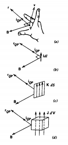
current I, or a surface with current per unit length K, or over a volume with current per unit area J, we use the differential sized current elements, as in Figures 5-7b-5-7d:

\[dq \textbf{v} = \left \{ \begin{matrix} \textbf{I} dl & \textrm{(line current)} \\ \textbf{K} dS & \textrm{(surface current)} \\ \textbf{J} dV & \textrm{(volume current)} \end{matrix} \right. \]

The total magnetic field for a current distribution is then obtained by integrating the contributions from all the incremental elements:

\[\textbf{B} = \left \{ \begin{matrix} \dfrac{\mu_{0}}{4 \pi} \int_{L} \dfrac{\textbf{I} dl \times \textbf{i}_{QP}}{r^{2}_{QP}} & \textrm{(line current)} \\ \dfrac{\mu_{0}}{4 \pi} \int_{S} \dfrac{\textbf{K} dS \times \textbf{i}_{QP}}{r^{2}_{QP}} & \textrm{(surface current)} \\ \dfrac{\mu_{0}}{4 \pi} \int_{V} \dfrac{\textbf{J} dV \times \textbf{i}_{QP}}{r^{2}_{QP}} & \textrm{(volume current)} \end{matrix} \right. \]

The direction of the magnetic field due to a current element is found by the right-hand rule, where if the forefinger of the right hand points in the direction of current and the middle finger in the direction of the field point, then the thumb points in the direction of the magnetic field. This magnetic field B can then exert a force on other currents, as given in Section 5-1-1.

5-2-2 Line Currents

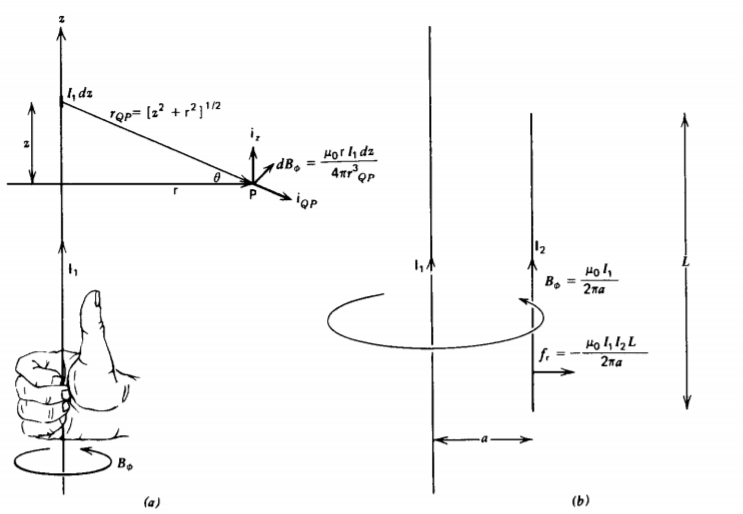
A constant current I₁ flows in the z direction along a wire of infinite extent, as in Figure 5-8a. Equivalently, the right-hand rule allows us to put our thumb in the direction of current. Then the fingers on the right hand curl in the direction of B, as shown in Figure 5-8a. The unit vector in the direction of the line joining an incremental current element I₁ dz at z to a field point P is

\[\textbf{i}_{QP} = \textbf{i}_{\textrm{r}} \cos \theta - \textbf{i}_{z} \sin \theta = \textbf{i}_{r} \dfrac{\textrm{r}}{r_{QP}} - \textbf{i}_{z} \dfrac{z}{r_{QP}} \]

Figure 5-8 (a) The magnetic field due to an infinitely long z-directed line current is in the \(\phi\) direction. (b) Two parallel line currents attract each other if flowing in the same direction and repel if oppositely directed.

with distance

\[r_{QP} = (z^{2} + \textrm{r}^{2})^{1/2} \]

The magnetic field due to this current element is given by (4) as

\[d \textbf{B} = \dfrac{\mu_{0}}{4 \pi} \dfrac{I_{1} dz (\textbf{i}_{z} \times \textbf{i}_{QP})}{r^{2}_{QP}} = \dfrac{\mu_{0}I_{1} \textrm{r} dz}{4 \pi (z^{2} + \textrm{r}^{2})^{3/2}} \textbf{i}_{\phi} \]

The total magnetic field from the line current is obtained by integrating the contributions from all elements:

\[B_{\phi} = \dfrac{\mu_{0} I_{1} \textrm{r}}{4 \pi} \int_{- \infty}^{+ \infty} \dfrac{dz}{(z^{2} + \textrm{r}^{2})^{3/2}} \\ = \dfrac{\rho_{0} I_{1} \textrm{r}}{4 \pi} \dfrac{z}{\textrm{r}^{2} (z^{2} + \textrm{r}^{2})^{1/2}} \bigg|_{z = - \infty}^{+ \infty} \\ = \dfrac{\mu_{0} I_{1}}{2 \pi \textrm{r}} \]

If a second line current \(I_{2}\) of finite length L is placed at a distance a and parallel to I₁, as in Figure 5-8b, the force on \(I_{1}\) due to the magnetic field of \(I_{1}\) is

\[\textbf{f} = \int_{-L/2}^{+L/2} I_{2} dz \textbf{i}_{z} \times \textbf{B} \\ int_{-L/2}^{+L/2} I_{2} dz \dfrac{\mu_{0}I_{1}}{2 \pi a} (\textbf{i}_{z} \times \textbf{i}_{\phi}) \\ = - \dfrac{\mu_{0} I_{1} I_{2} L}{2 \pi a } \textbf{i}_{r} \]

If both currents flow in the same direction (\(I_{1}I_{2} >0 \)), the force is attractive, while if they flow in opposite directions (\(I_{1} I_{2} <0\)), the force is repulsive. This is opposite in sense to the Coulombic force where opposite charges attract and like charges repel.

5-2-3 Current Sheets

(a) Single Sheet of Surface Current

A constant current \(K_{0} \textbf{i}_{z}\), flows in the y =0 plane, as in Figure 5-9a. We break the sheet into incremental line currents \(K_{0} dx\), each of which gives rise to a magnetic field as given by (8). From Table 1-2, the unit vector \(\textbf{i}_{\phi}\) is equivalent to the Cartesian components

\[\textbf{i}_{\phi} = - \sin \phi \textbf{i}_{x} + \cos \phi \textbf{i}_{y} \]

Figure 5-9 (a) A uniform surface current of infinite extent generates a uniform magnetic field oppositely directed on each side of the sheet. The magnetic field is perpendicular to the surface current but parallel to the plane of the sheet. (b) The magnetic field due to a slab of volume current is found by superimposing the fields due to incremental surface currents. (c) Two parallel but oppositely directed surface current sheets have fields that add in the region between the sheets but cancel outside the sheet. (d) The force on a current sheet is due to the average field on each side of the sheet as found by modeling the sheet as a uniform volume current distributed over an infinitesimal thickness \(\Delta\).

Figure 5-9

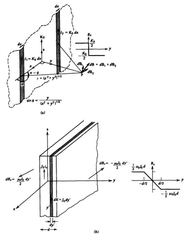
The symmetrically located line charge elements a distance x on either side of a point P have y magnetic field components that cancel but x components that add. The total magnetic field is then

\[B_{x} = - \int_{- \infty}^{+ \infty} \dfrac{\mu_{0} K_{0} \sin \phi}{2 \pi (x^{2} + y^{2})^{1/2}} dx \\ = \dfrac{- \mu_{0} K_{0}y}{2 \pi} \int_{-infty}^{+ \infty} \dfrac{dx}{(x^{2} + y^{2})} \\ = \dfrac{- \mu_{0} K_{0}}{2 \pi} \tan^{-1} \dfrac{x}{y} \bigg|_{- \infty}^{+ \infty} \\ = \left \{ \begin{matrix} - \mu_{0} K_{0}/2, & y > 0 \\ \mu_{0}K_{0}/2, & y < 0 \end{matrix} \right. \]

The field is constant and oppositely directed on each side of the sheet.

(b) Slab of Volume Current

If the z-directed current \(J_{0} \textbf{i}_{z}\) is uniform over a thickness d, as in Figure 5-9b, we break the slab into incremental current sheets \(J_{0} dy'\). The magnetic field from each current sheet is given by (11). When adding the contributions of all the differential-sized sheets, those to the left of a field point give a negatively x directed magnetic field while those to the right contribute a positively x-directed field:

\[B_{x} = \left \{ \begin{matrix} \int_{-d/2}^{+d/2} \dfrac{- \mu_{0} J_{0} dy'}{2} = \dfrac{- \mu_{0} J_{0} d}{2}, & y > \dfrac{d}{2} \\ \int_{-d/2}^{+d/2} \dfrac{mu_{0}J_{0}dy'}{2} = \dfrac{\mu_{0}J_{0}d}{2}, & y < - \dfrac{d}{2} \\ \int_{-d/2}^{y} \dfrac{- mu_{0}J_{0} dy'}{2} + \int_{y}^{d/2} \dfrac{mu_{0}J_{0}dy'}{2} = - \mu_{0} J_{0}y, & - \dfrac{d}{2} \leq y \leq \dfrac{d}{2} \end{matrix} \right. \]

The total force per unit area on the slab is zero:

\[F_{Sy} = \int_{-d/2}^{+d/2} J_{0}B_{x} dy = - \mu_{0}J_{0}^{2} \int_{-d/2}^{+d/2} y dy \\ = - \mu_{0} J_{0}^{2} \dfrac{y^{2}}{2} \bigg|_{-d/2}^{+d/2} = 0 \]

A current distribution cannot exert a net force on itself.

(c) Two Parallel Current Sheets

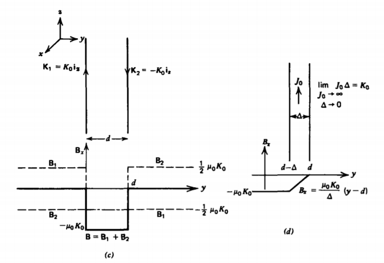
If a second current sheet with current flowing in the opposite direction \(K_{0} \textbf{i}_{z}\) is placed at y = d parallel to a current sheet \(K_{0} \textbf{i}_{z}\) at y = 0, as in Figure 5-9c, the magnetic field due to each sheet alone is

\[\textbf{B}_{1} = \left \{ \begin{matrix} \dfrac{- \mu_{0} K_{0}}{2} \textbf{i}_{x}, & y>0 \\ \dfrac{\mu_{0}K_{0}}{2} \textbf{i}_{x}, & y< 0 \end{matrix} \right. \: \textbf{B}_{2} = \left \{ \begin{matrix} \dfrac{\mu_{0}K_{0}}{2} \textbf{i}_{x}, & y > d \\ \dfrac{- \mu_{0}K_{0}}{2} \textbf{i}_{x}, & y < d \end{matrix} \right. \]

Thus in the region outside the sheets, the fields cancel while they add in the region between:

\[\textbf{B} = \textbf{B}_{1} + \textbf{B}_{2} = \left \{ \begin{matrix} - \mu_{0} K_{0} \textbf{i}_{x}, & 0 < y < d \\ 0, & y < 0, y> d \end{matrix} \right. \]

The force on a surface current element on the second sheet is

\[\textbf{df} = - K_{0} \textbf{i}_{z} d \textrm{S} \times \textbf{B} \]

However, since the magnetic field is discontinuous at the current sheet, it is not clear which value of magnetic field to use. To take the limit properly, we model the current sheet at y = d as a thin volume current with density \(J_{0}\) and thickness \(\Delta\), as in Figure 5-9d, where \(K_{0} = J_{0} \Delta\).

The results of (12) show that in a slab of uniform volume current, the magnetic field changes linearly to its values at the surfaces

\[B_{x} (y = d - \Delta) = - \mu_{0} K_{0} \\ B_{x} (y = d) = 0 \]

so that the magnetic field within the slab is

\[B_{x} = \dfrac{\mu_{0}K_{0}}{\Delta} (y-d) \]

The force per unit area on the slab is then

\[\textbf{F}_{S} = - \int_{d - \Delta}^{d} \dfrac{\mu_{0}K_{0}}{\Delta} J_{0}(y-d) \textbf{i}_{y} dy \\ = \dfrac{- \mu_{0}K_{0}J_{0}}{\Delta} \dfrac{(y-d)^{2}}{2} \textbf{i}_{y} \big| _{d - \Delta}^{d} \\ = \dfrac{\mu_{0}K_{0}J_{0}\Delta}{2} \textbf{i}_{y} = \dfrac{\mu_{0} K_{0}^{2}}{2} \textbf{i}_{y} \]

The force acts to separate the sheets because the currents are in opposite directions and thus repel one another.

Just as we found for the electric field on either side of a sheet of surface charge in Section 3-9-1, when the magnetic field is discontinuous on either side of a current sheet K, being B₁ on one B₂ side and on the other, the average magnetic field is used to compute the force on the sheet:

\[\textbf{df}= \textbf{K} d \textrm{S} \times \dfrac{(\textbf{B}_{1} + \textbf{B}_{2})}{2} \]

In our case

\[\textbf{B}_{1} = - \mu_{0} K_{0} \textbf{i}_{x}, \: \: \: \textbf{B}_{2} = 0 \]

5-2-4 Hoops of Line Current

(a) Single hoop

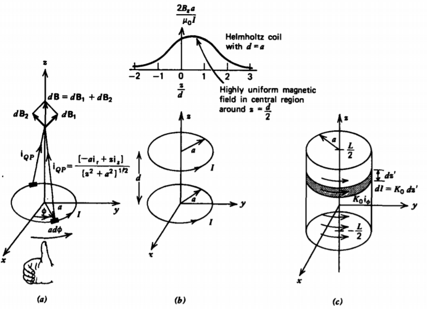
A circular hoop of radius a centered about the origin in the xy plane carries a constant current I, as in Figure 5-10a. The distance from any point on the hoop to a point at z along the z axis is

\[r_{QP} = (z^{2} + a^{2})^{1/2} \]

in the direction

\[\textbf{i}_{QP} = \dfrac{(-a \textbf{i}_{\textrm{r}} + z \textbf{i}_{z})}{(z^{2} + a^{2})^{1/2}} \]

Figure 5-10 (a) The magnetic field due to a circular current loop is z directed along the axis of the hoop. (b) A Helmholtz coil, formed by two such hoops at a distance apart d equal to their radius, has an essentially uniform field near the center at z = d/2. (c) The magnetic field on the axis of a cylinder with a \(\phi\)-directed surface current is found by integrating the fields due to incremental current loops.

so that the incremental magnetic field due to a current element of differential size is

\[d \textbf{B} = \dfrac{\mu_{0}}{4 \pi r^{2}_{QP}} Ia d \phi \textbf{i}_{\phi} \times \textbf{i}_{QP} \\ = \dfrac{\mu_{0}Ia d \phi}{4 \pi (z^{2} + a^{2})^{3/2}} (a \textbf{i}_{z} + z \textbf{i}_{\textrm{r}}) \]

The radial unit vector changes direction as a function of \(\phi\), being oppositely directed at -\(\phi\), so that the total magnetic field due to the whole hoop is purely z directed:

\[B_{z} = \dfrac{\mu_{0} Ia^{2}}{4 \pi (z^{2} + a^{2})^{3/2}} \int_{0}^{2 \pi} d \phi \\ = \dfrac{\mu_{0} Ia^{2}}{2 (z^{2} + a^{2})^{3/2}} \]

The direction of the magnetic field can be checked using the right-hand rule. Curling the fingers on the right hand in the direction of.the current puts the thumb in the direction of the magnetic field. Note that the magnetic field along the z axis is positively z directed both above and below the hoop.

(b) Two Hoops (Hehnholtz Coil)

Often it is desired to have an accessible region in space with an essentially uniform magnetic field. This can be arranged by placing another coil at z = d, as in Figure 5-1 Ob. Then the total magnetic field along the z axis is found by superposing the field of (25) for each hoop:

\[\textbf{B}_{z} = \dfrac{\mu_{0} Ia^{2}}{2} \bigg( \dfrac{1}{(z^{2} + a^{2})^{3/2}} + \dfrac{1}{((z - d)^{2} + a^{2})^{3/2}} \bigg) \]

We see then that the slope of \(B_{z}\),

\[\dfrac{\partial B_{z}}{\partial z} = \dfrac{3 \mu_{0} Ia^{2}}{2} \bigg( \dfrac{-z}{(z^{2} + a^{2})^{5/2}} - \dfrac{(z-d)}{((z-d)^{2} + a^{2})^{5/2}} \bigg) \]

is zero at z = d/2. The second derivative,

\[\dfrac{\partial^{2}B_{z}}{\partial z^{2}} = \dfrac{ 3 \mu_{0}I a^{2}}{2} \bigg( \dfrac{5z^{2}}{(z^{2} + a^{2})^{7/2}} - \dfrac{1}{(z^{2} + a^{2})^{5/2}} + \dfrac{5 (z-d)^{2}}{((z-d)^{2} + a^{2})^{7/2}} - \dfrac{1}{((z-d)^{2} + a^{2})^{5/2}} \bigg) \]

can also be set to zero at z = d/2, if d = a, giving a highly uniform field around the center of the system, as plotted in Figure 5-10b. Such a configuration is called a Helmholtz coil.

(c) Hollow Cylinder of Surface Current

A hollow cylinder of length L and radius a has a uniform surface current \(K_{0} \textbf{i}_{\phi}\) as in Figure 5-10c. Such a configuration is arranged in practice by tightly winding N turns of a wire around a cylinder and imposing a current I through the wire. Then the current per unit length is

\[K_{0} = NI/L \]

The magnetic field along the z axis at the position z due to each incremental hoop at z' is found from (25) by replacing z by (z - z' ) and I by \(K_{0} dz'\):

\[d B_{z} = \dfrac{ \mu_{0} a^{2} K_{0} dz'}{2 [(z-z')^{2} + a^{2}]^{3/2}} \]

The total axial magnetic field is then

\[B_{z} = \int_{z' = -L/2}^{+ L/2} \dfrac{\mu_{0} a^{2} K_{0}}{2} \dfrac{dz'}{[(z-z')^{2} + a^{2}]^{3/2}} \\ = \dfrac{\mu_{0}a^{2} K_{0}}{2} \dfrac{(z'-z)}{a^{2} [(z-z')^{2} + a^{2}]^{1/2}} \bigg|_{z' = -L/2}^{+L/2} \\ = \dfrac{\mu_{0}K_{0}}{2} \bigg( \dfrac{-z + L/2}{[(z-L/2)^{2} + a^{2}]^{1/2}} + \dfrac{z + L/2}{[(z + L/2)^{2} + a^{2}]^{1/2}} \bigg) \]]

As the cylinder becomes very long, the magnetic field far from the ends becomes approximately constant

\[\lim_{L \rightarrow \infty} B_{z} = \mu_{0} K_{0} \]