5.3: Divergence and Curl of the Magnetic Field

Because of our success in examining various vector operations on the electric field, it is worthwhile to perform similar operations on the magnetic field. We will need to use the following vector identities from Section 1-5-4, Problem 1-24 and Sections 2-4-1 and 2-4-2:

\[\nabla \cdot (\nabla \times \textbf{A}) = 0 \]

\[\nabla \times (\nabla f) = 0 \]

\[\nabla \bigg( \frac{1}{r_{QP}}) = - \frac{\textbf{i}_{QP}}{r^{2}_{QP}} \]

\[\int_{V} \nabla^{2} \bigg( \frac{1}{r_{QP}} \bigg) d \textrm{V} = \left \{ \begin{matrix} 0, & r_{QP} \neq 0 \\ -4 \pi , & r_{QP} = 0 \end{matrix} \right. \]

\[\nabla \cdot (\textbf{A} \times \textbf{B}) = \textbf{B} \cdot (\nabla \times \textbf{A}) - \textbf{A} \cdot \nabla \times \textbf{B} \]

\[\nabla \times (\textbf{A} \times \textbf{B}) = (\textbf{B} \cdot \nabla)\textbf{A} - (\textbf{A} \cdot \nabla) \textbf{B} + (\nabla \cdot \textbf{B} \textbf{A} - (\nabla \cdot \textbf{A}) \textbf{B} \]

\[\nabla (\textbf{A} \cdot \textbf{B}) = (\textbf{A} \cdot \nabla) \textbf{B} + (\textbf{B} \cdot \nabla) \textbf{A} + \textbf{A} \times (\nabla \times \textbf{B}) + \textbf{B} \times (\nabla \times \textbf{A}) \]

5-3-1 Gauss' Law for the Magnetic Field

Using (3) the magnetic field due to a volume distribution of current J is rewritten as

\[\textbf{B} = \frac{\mu_{0}}{4 \pi} \int_{\textrm{V}} \frac{\textbf{J} \times \textbf{i}_{QP}}{r^{2}_{QP}} d \textrm{V} = \frac{-\mu_{0}}{4 \pi} \int_{\textrm{V}} \textbf{J} \times \nabla \bigg( \frac{1}{r_{QP}} \bigg) d \textrm{V} \]

If we take the divergence of the magnetic field with respect to field coordinates, the del operator can be brought inside the integral as the integral is only over the source coordinates:

\[\nabla \cdot \textbf{B} = \frac{-\mu_{0}}{4 \pi} \int_{\textrm{V}} \nabla \cdot \bigg[ \textbf{J} \times \nabla \bigg( \frac{1}{r_{QP}} \bigg) \bigg] d \textrm{V} \]

The integrand can be expanded using (5)

\[\nabla \cdot \bigg[ \textbf{J} \times \nabla \bigg( \frac{1}{r_{QP}} \bigg) \bigg] = \nabla \bigg(\frac{1}{r_{QP}} \bigg) \cdot \underbrace{(\nabla \times \textbf{J})}_{0} - \textbf{J} \cdot \underbrace{\nabla \times \bigg[ \nabla \bigg( \frac{1}{r_{QP}} \bigg) \bigg]}_{0} = 0 \]

The first term on the right-hand side in (10) is zero because J is not a function of field coordinates, while the second term is zero from (2), the curl of the gradient is always zero. Then (9) reduces to

\[\nabla \cdot \textbf{B} = 0 \]

This contrasts with Gauss's law for the displacement field where the right-hand side is equal to the electric charge density. Since nobody has yet discovered any net magnetic charge, there is no source term on the right-hand side of (11).

The divergence theorem gives us the equivalent integral representation

\[\int_{\textrm{V}} \nabla \cdot \textbf{B} d \textrm{V} = \oint_{S} \textbf{B} \cdot \textbf{B} \cdot \textbf{dS} = 0 \]

which tells us that the net magnetic flux through a closed surface is always zero. As much flux enters a surface as leaves it. Since there are no magnetic charges to terminate the magnetic field, the field lines are always closed

5-3-2 Ampere's Circuital Law

We similarly take the curl of (8) to obtain

\[\nabla \times \textbf{B} = \frac{-\mu_{0}}{4 \pi} \int_{\textrm{V}} \nabla \times \bigg[ \textbf{J} \times \nabla \bigg( \frac{1}{r_{QP}} bigg) \bigg] d \textrm{V} \]

where again the del operator can be brought inside the integral and only operates on \(r_{QP}\)

We expand the integrand using (6):

\[\nabla \times \bigg[ \textbf{J} \times \nabla \bigg( \frac{1}{r_{QP}} \bigg) \bigg] = \bigg[ \nabla \bigg( \frac{1}{r_{QP}} \bigg) \underbrace{\cdot \bigg] \textbf{J}}_{0} - ( \textbf{J} \cdot \nabla) \nabla \bigg( \frac{1}{r_{QP}} \bigg) \\ + \bigg[ \nabla^{2} \bigg( \frac{1}{r_{QP}} \bigg) \bigg] \textbf{J} - \underbrace{(\nabla \cdot \textbf{J}) \nabla}_{0} \bigg(\frac{1}{r_{QP}}\bigg) \]

where two terms on the right-hand side are zero because J is not a function of the field coordinates. Using the identity of (7)

\[\nabla \bigg[ \textbf{J} \cdot \nabla \bigg( \frac{1}{r_{QP}} \bigg) \bigg] = \bigg[ \nabla \bigg( \frac{1}{r_{QP}} \bigg) \underbrace{\cdot \nabla \bigg] \textbf{J}}_{0} + ( \textbf{J} \cdot \nabla ) \nabla \bigg(\frac{1}{r_{QP}}\bigg) \\ + \nabla \bigg( \frac{1}{r_{QP}} \bigg) \times \underbrace{(\nabla \times \textbf{J})}_{0} + \textbf{J} \times \bigg[ \underbrace{\nabla \times \nabla \bigg( \frac{1}{r_{QP}} \bigg)}_{0} \bigg] \]

the second term on the right-hand side of (14) can be related to a pure gradient of a quantity because the first and third terms on the right of (15) are zero since J is not a function of field coordinates. The last term in (15) is zero because the curl of a gradient is always zero. Using (14) and (15), (13) can be rewritten as

\[\nabla \times \textbf{B} = \frac{\mu_{0}}{4 \pi} \int_{\textrm{V}} \{ \nabla \bigg[ \textbf{J} \cdot \nabla \bigg( \frac{1}{r_{QP}} \bigg) \bigg] - \textbf{K} \nabla^{2} \bigg( \frac{1}{r_{QP}} \bigg) \} d \textrm{V} \]

Using the gradient theorem, a corollary to the divergence theorem, (see Problem 1-15a), the first volume integral is converted to a surface integral

\[\nabla \times \textbf{B} = \frac{\mu_{0}}{4 \pi} \bigg[ \int_{S} \underbrace{\textbf{J} \cdot \nabla \bigg( \frac{1}{r_{QP}} \bigg) \textbf{dS}}_{0} - \int_{\textrm{V}} \textbf{J} \nabla^{2} \bigg(\frac{1}{r_{QP}} \bigg) d \textrm{V} \bigg] \]

This surface completely surrounds the current distribution so that S is outside in a zero current region where J =0 so that the surface integral is zero. The remaining volume integral is nonzero only when \(r_{QP}\) =0, so that using (4) we finally obtain

\[\nabla \times \textbf{B} = \mu_{0} \textbf{J} \]

which is known as Ampere's law.

Stokes' theorem applied to (18) results in Ampere's circuital law:

\[\int_{S} \nabla \times \frac{\textbf{B}}{\mu_{0}} \cdot \textbf{dS} = \oint_{L} \frac{\textbf{B}}{\mu_{0}} \cdot \textbf{dL} = \int_{S} \textbf{J} \cdot \textbf{dS} \]

Like Gauss's law, choosing the right contour based on symmetry arguments often allows easy solutions for B.

If we take the divergence of both sides of (18), the left-hand side is zero because the divergence of the curl of a vector is always zero. This requires that magnetic field systems have divergence-free currents so that charge cannot accumulate. Currents must always flow in closed loops.

5-3-3 Currents With Cylindrical Symmetry

A surface current \(K_{0} \textbf{i}_{z}\) flows on the surface of an infinitely long hollow cylinder of radius a. Consider the two symmetrically located line charge elements \(dI = K_{0} a d \phi\) and their effective fields at a point P in Figure 5-11a. The magnetic field due to both current elements cancel in the radial direction but add in the \(\phi\) direction. The total magnetic field can be found by doing a difficult integration over \(\phi\). However

Figure 5-11 (a) The magnetic field of an infinitely long cylinder carrying a surface current parallel to its axis can be found using the Biot-Savart law for each incremental line current element. Symmetrically located elements have radial field components that cancel but \(\phi\) field components that add. (b) Now that we know that the field is purely \(\phi\) directed, it is easier to use Ampere's circuital law for a circular contour concentric with the cylinder. For r<a no current passes through the contour while for r> a all the current passes through the contour. (c) If the current is uniformly distributed over the cylinder the smaller contour now encloses a fraction of the current.

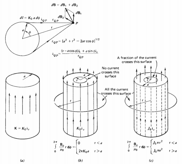
using Ampere's circuital law of (19) is much easier. Since we know the magnetic field is \(\phi\) directed and by symmetry can only depend on r and not \(\phi\) or z, we pick a circular contour of constant radius r as in Figure 5-11 b. Since \(\textbf{dl} = r d \phi \textbf{i}_{\phi}\) is in the same direction as B, the dot product between the magnetic field and dl becomes a pure multiplication. For r<a no current passes through the surface enclosed by the contour, while for r > a all the current is purely perpendicular to the normal to the surface of the contour:

\[\oint_{L} \frac{\textbf{B}}{\mu_{0}} \cdot \textbf{dl} = \int_{0}^{2 \pi} \frac{B_{\phi}}{\mu_{0}} \textrm{r} d \phi = \frac{2 \pi \textrm{r} B_{\phi}}{\mu_{0}} = \left \{ \begin{matrix} K_{0} 2 \pi a = I, & \textrm{r} > a \\ 0, & \textrm{r} < a \end{matrix} \right. \]

where I is the total current on the cylinder.

The magnetic field is thus

\[B_{\phi} = \left \{ \begin{matrix} \mu_{0} K_{0} a/r = \mu_{0} I/(2 \pi r), & r>a \\ 0, & r<a \end{matrix} \right. \]

Outside the cylinder, the magnetic field is the same as if all the current was concentrated along the axis as a line current.

(b) Volume Current

If the cylinder has the current uniformly distributed over the volume as \(J_{0} \textbf{i}_{z}\) the contour surrounding the whole cylinder still has the total current \(I = J_{0} \pi a^{2}\) passing through it. If the contour has a radius smaller than that of the cylinder, only the fraction of current proportional to the enclosed area passes through the surface as shown in Figure 5-11c:

\[\oint_{L} \frac{B_{\phi}}{\mu_{0}} \textrm{r} \d \phi = \frac{2 \pi \textrm{r} B_{\phi}}{\mu_{0}} = \left \{ \begin{matrix} J_{0} \pi a^{2} = I, & \textrm{r} >a \\ J_{0} \pi \textrm{r}^{2} = I \textrm{r}^{2}/a^{2}, & \textrm{r} < a \end{matrix} \right. \]

so that the magnetic field is

\[B_{\phi} = \left \{ \begin{matrix} \frac{\mu_{0} J_{0} a^{2}}{2 \textrm{r}} = \frac{\mu_{0}I}{2 \pi \textrm{r}}, & \textrm{r} > a \\ \frac{\mu_{0} J_{0} \textrm{r}}{2} = \frac{\mu_{0}I \textrm{r}}{2 \pi a^{2}}, & \textrm{r} < a \end{matrix} \right. \]