5.4: The Vector Potential

Uniqueness

Since the divergence of the magnetic field is zero, we may write the magnetic field as the curl of a vector,

\[\nabla \cdot \textbf{B} = 0 \Rightarrow \textbf{B} = \nabla \times \textbf{A} \label{1} \]

where A is called the vector potential, as the divergence of the curl of any vector is always zero. Often it is easier to calculate A and then obtain the magnetic field from Equation \ref{1}.

From Ampere's law, the vector potential is related to the current density as

\[\nabla \times \textbf{B} = \nabla \times (\nabla \times \textbf{A}) = \nabla (\nabla \cdot \textbf{A}) - \nabla^{2} \textbf{A} = \mu_{0} \textbf{J} \]

We see that (1) does not uniquely define A, as we can add the gradient of any term to A and not change the value of the magnetic field, since the curl of the gradient of any function is always zero:

\[\textbf{B} \rightarrow \textbf{A} + \nabla f \Rightarrow \textbf{B} = \nabla \times ( \textbf{A} + \nabla f ) = \nabla \times \textbf{A} \]

Helmholtz's theorem states that to uniquely specify a vector, both its curl and divergence must be specified and that far from the sources, the fields must approach zero. To prove this theorem, let's say that we are given, the curl and divergence of A and we are to determine what A is. Is there any other vector C, different from A that has the same curl and divergence? We try C of the form

\[\textbf{C} = \textbf{A} + \textbf{a} \]

and we will prove that a is zero.

By definition, the curl of C must equal the curl of A so that the curl of a must be zero:

\[\nabla \times \textbf{C} = \nabla \times (\textbf{A} + \textbf{a}) = \nabla \times \textbf{A} \Rightarrow \nabla \times \textbf{a} = 0 \]

This requires that a be derivable from the gradient of a scalar function f

\[\nabla \times \textbf{a} = 0 \Rightarrow \textbf{a} = \nabla f \]

Similarly, the divergence condition requires that the divergence of a be zero,

\[\nabla \cdot \textbf{C} = \nabla \cdot (\textbf{A} + \textbf{a}) = \nabla \cdot \textbf{A} \Rightarrow \nabla \cdot \textbf{a} = 0 \]

so that the Laplacian of \(f\) must be zero,

\[\nabla \cdot \textbf{a} = \nabla^{2} f = 0 \]

In Chapter 2 we obtained a similar equation and solution for the electric potential that goes to zero far from the charge distribution:

\[\nabla^{2} V = - \frac{\rho}{\varepsilon} \Rightarrow V = \int_{\textrm{V}} \frac{\rho d \textrm{V}}{4 \pi \varepsilon r_{QP}} \]

If we equate f to V, then \(\rho\) must be zero giving us that the scalar function f is also zero. That is, the solution to Laplace's equation of (8) for zero sources everywhere is zero, even though Laplace's equation in a region does have nonzero solutions if there are sources in other regions of space. With f zero, from (6) we have that the vector a is also zero and then C = A, thereby proving Helmholtz's theorem.

5-4-2 The Vector Potential of a Current Distribution

Since we are free to specify the divergence of the vector potential, we take the simplest case and set it to zero:

\[\nabla \cdot \textbf{A} = 0 \]

Then (2) reduces to

\[\nabla^{2} \textbf{A} = - \mu_{0} \textbf{J} \]

Each vector component of (11) is just Poisson's equation so that the solution is also analogous to (9)

\[\textbf{A} = \frac{\mu_{0}}{4 \pi} \int_{\textrm{V}} \frac{\textbf{J} d \textrm{V}}{r_{QP}} \]

The vector potential is often easier to use since it is in the same direction as the current, and we can avoid the often complicated cross product in the Biot-Savart law. For moving point charges, as well as for surface and line currents, we use (12) with the appropriate current elements:

\[\textbf{J} d \textrm{V} \rightarrow \textbf{K} d \textrm{S} \rightarrow \textbf{I} dL \rightarrow q \textbf{v} \]

5-4-3 The Vector Potential and Magnetic Flux

Using Stokes' theorem, the magnetic flux through a surface can be expressed in terms of a line integral of the vector potential:

\[\begin{align*} \Phi &= \int_{S} \textbf{B} \cdot \textbf{dS} \\[4pt] &= \int_{S} \nabla \times \textbf{A} \cdot \textbf{dS} \\[4pt] &= \oint_{L} \textbf{A} \cdot \textbf{dl} \end{align*} \] \[\]

(a) Finite Length Line Current

The problem of a line current \(I\) of length \(L\), as in Figure 5-12a appears to be nonphysical as the current must be continuous. However, we can imagine this line current to be part of a closed loop and we calculate the vector potential and magnetic field from this part of the loop.

Figure 5-12 (a) The magnetic field due to a finite length line current is most easily found using the vector potential, which is in the direction of the current. This problem is physical only if the line current is considered to be part of a closed loop. (b) The magnetic field from a length \(w\) of surface current is found by superposing the vector potential of (a) with \(L \rightarrow \infty\). The field lines are lines of constant \(A_{z}\) (c) The magnetic flux through a square current loop is in the -x direction by the right-hand rule.

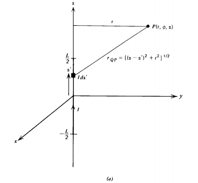
The distance \(r_{QP}\) from the current element \(I \: dz'\) to the field point at coordinate (r, \(\phi\), z) is

\[r_{QP} = [ (z-z')^{2} + \textrm{r}^{2}]^{1/2} \]

The vector potential is then

\[\begin{align*} A_{z} &= \frac{\mu_{0}I}{4 \pi} \int_{-L/2}^{L/2} \frac{dz'}{[(z-z')^{2} + \textrm{r}^{2}]^{1/2}} \\[4pt] &= \frac{\mu_{0}I}{4 \pi} \ln \left( \frac{-z + L/2 + [(z-L/2)^{2} + \textrm{r}^{2}]^{1/2}}{-(z+L/2) + [(z + L/2)^{2} + \textrm{r}^{2}]^{1/2}} \right) \\[4pt] &= \frac{\mu_{0}I}{4 \pi} \left(\sinh^{-1} \frac{-z + L/2}{\textrm{r}} + \sinh^{-1} \frac{z + L/2}{\textrm{r}} \right) \end{align*} \] \[\]

with associated magnetic field

\[ \begin{align*} \textbf{B} &= \nabla \times \textbf{A} \\[4pt] &= \left( \frac{1}{\textrm{r}} \frac{\partial A_{z}}{\partial \phi} - \frac{\partial A_{\phi}}{dz} \right) \textbf{i}_{\textrm{r}} + \left( \frac{\partial A_{\textrm{r}}}{\partial z} - \frac{\partial A_{z}}{\partial \textrm{r}} \right) \textbf{i}_{\phi} + \frac{1}{\textrm{r}} \left( \frac{\partial}{\partial \textrm{r}} (\textrm{r} A_{\phi}) - \frac{\partial A_{\textrm{r}}}{\partial \phi} \right) \textbf{i}_{z} \\[4pt] &= - \frac{\partial A_{z}}{\partial \textrm{r}} \textbf{i}_{\phi} \\[4pt] &= \frac{- \mu_{0} I \textrm{r}}{4 \pi} \left( \frac{1}{[(z-L/2)^{2} + \textrm{r}^{2}]^{1/2} ( -z + L/2 + [(z-L/2)^{2} + \textrm{r}^{2}]^{1/2} )} - \frac{1}{[(z+L/2)^{2} + \textrm{r}^{2}]^{1/2} (-(z-L/2) + [(z + L/2)^{2} + \textrm{r}^{2}]^{1/2} ) } \right) \textbf{i}_{\phi} \\[4pt] &= \frac{\mu_{0}I}{4 \pi \textrm{r}} \left( \frac{-z + L/2}{[\textrm{r}^{2} + (z-L/2)^{2}]^{1/2}} + \frac{z + L/2}{[\textrm{r}^{2} + (z + L/2)^{2}]^{1/2}} \right) \textbf{i}_{\phi} \end{align*} \] \[ \]

Figure 5-12

For large \(L\), (17) approaches the field of an infinitely long line current as given in Section 5-2-2:

\[\lim_{L \rightarrow \infty} \left \{ \begin{matrix} A_{z} = \frac{- \mu_{0}I}{2 \pi} \ln \textrm{r} + \textrm{const} \\ B_{\phi} = - \frac{\partial A_{z}}{\partial \textrm{r}} = \frac{\mu_{0} I}{2 \pi \textrm{r}} \end{matrix} \right. \]

Note that the vector potential constant in (18) is infinite, but this is unimportant as this constant has no contribution to the magnetic field.

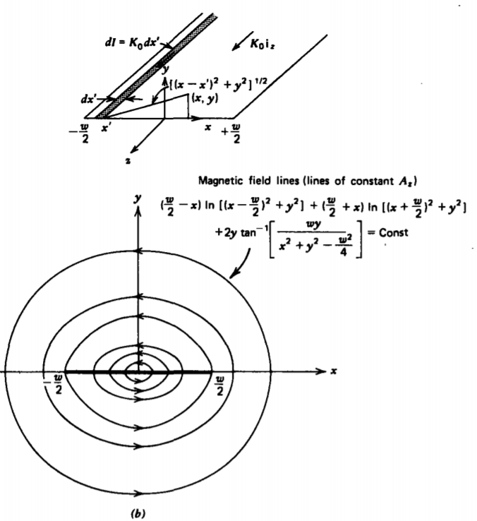
(b) Finite Width Surface Current

If a surface current \(K_{0} \text{i}_{z}\) of width \(w\), is formed by laying together many line current elements, as in Figure 5-12b, the vector potential at (x, y) from the line current element \(K_{0} dx'\) at position x' is given by (18):

\[dA_{z} = \frac{- \mu_{0} K_{0} dx'}{4 \pi} \ln [(x-x')^{2} + y^{2}] \]

The total vector potential is found by integrating over all elements:

\[A_{z} = \frac{-\mu_{0}K_{0}}{4 \pi} \int_{-w/2}^{+w/2} \ln [(x-x')^{2} + y^{2}]dx' \\ = \frac{-\mu_{0}K_{0}}{4 \pi} \left( (x'-x) \ln [(x-x')^{2} + y^{2}]-2(x'-x) \\ = 2y \tan^{-1} \frac{(x'-x)}{y}\right) \bigg|_{-w/2}^{+w/2} \\ = \frac{-\mu_{0}K_{0}}{4 \pi} \left( \left( \frac{w}{2} - x \right) \ln \bigg[ \left( x - \frac{w}{2} \right)^{2} + y^{2} \bigg] \\ + \left( \frac{w}{2} + x \right) \ln \bigg[ \left( x + \frac{w}{2} \right)^{2} + y^{2} \bigg] \\ -2 w + 2 y \tan^{-1} \frac{wy}{y^{2} +x^{2} - w^{2}/4} \right) \]

*

The magnetic field is then

\[\textbf{B} = \textbf{i}_{x} \frac{\partial A_{z}}{\partial y} - \textbf{i}_{y} \frac{\partial A_{z}}{\partial x} \\ = \frac{- \mu_{0} K_{0}}{4 \pi} \left( 2 \tan^{-1} \frac{wy}{y^{2} + x^{2} - w^{2}/4} \textbf{i}_{x} + \ln \frac{(x + w/2)^{2} + y^{2}}{(x - w/2)^{2} + y^{2}} \textbf{i}_{y} \right) \]

The vector potential in two-dimensional geometries is also useful in plotting field lines,

\[\frac{dy}{dx} = \frac{B_{y}}{B_{x}} = \frac{- \partial A_{z}/ \partial x}{\partial A_{z} / \partial y} \]

for if we cross multiply (22),

\[\frac{\partial A_{z}}{\partial x} dx + \frac{\partial A_{z}}{\partial y} dy = d A_{z} = 0 \Rightarrow A_{z} = \textrm{const} \]

we see that it is constant on a field line. The field lines in Figure 5-12b are just lines of constant \(A_{z}\). The vector potential thus plays the same role as the electric stream function in Sections 4.3.2b and 4.4.3b.

\[\tan^{-1} (a-b) + \tan^{-1} (a + b) = \tan ^{-1} \frac{2a}{1-a^{2} + b^{2}} \nonumber \]

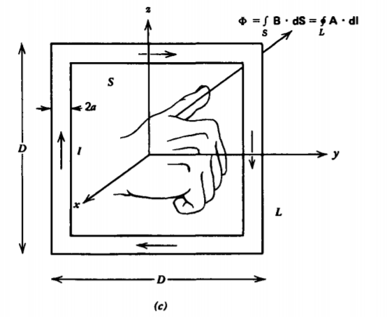
(c) Flux Through a Square Loop

The vector potential for the square loop in Figure 5-12c with very small radius a is found by superposing (16) for each side with each component of A in the same direction as the current in each leg. The resulting magnetic field is then given by four terms like that in (17) so that the flux can be directly computed by integrating the normal component of B over the loop area. This method is straightforward but the algebra is cumbersome

An easier method is to use (14) since we already know the vector potential along each leg. We pick a contour that runs along the inside wire boundary at small radius a. Since each leg is identical, we only have to integrate over one leg, then multiply the result by 4:

\begin{aligned}
\Phi= & 4 \int_{\substack{r=a \\
r=a / 2}}^{-a+D / 2} A_z d z \\
= & \frac{\mu_0 I}{\pi} \int_{a-D / 2}^{-a+D / 2}\left(\sinh ^{-1} \frac{-z+D / 2}{a}+\sinh ^{-1} \frac{z+D / 2}{a}\right) d z \\
= & \frac{\mu_0 I}{\pi}\left\{-\left(\frac{D}{2}-z\right) \sinh ^{-1} \frac{-z+D / 2}{a}+\left[\left(\frac{D}{2}-z\right)^2+a^2\right]^{1 / 2}\right. \\
& \left.+\left(\frac{D}{2}+z\right) \sinh ^{-1} \frac{z+D / 2}{a}-\left[\left(\frac{D}{2}+z\right)^2+a^2\right]^{1 / 2}\right\}\left.\right|_{a-D / 2} ^{-a+D / 2} \\
= & 2 \frac{\mu_0 I}{\pi}\left(-a \sinh ^{-1} 1+a \sqrt{2}+(D-a) \sinh ^{-1} \frac{D-a}{a}\right. \\
& \left.-\left[(D-a)^2+a^2\right]^{1 / 2}\right)
\end{aligned} \[\]

As \(a\) becomes very small, (24) reduces to

\[\lim_{a \rightarrow 0} \Phi = 2 \frac{\mu_{0}I}{\pi} D \left( \sinh^{-1} \left( \frac{D}{a} \right) - 1 \right) \]

We see that the flux through the loop is proportional to the current. This proportionality constant is called the self inductance and is only a function of the geometry:

\[L = \frac{\Phi}{I} = 2 \frac{\mu_{0}D}{\pi} \left( \sinh^{-1} \left( \frac{D}{a} \right) - 1 \right) \]

Inductance is more fully developed in Chapter 6.