5.5: Magnetization

Our development thus far has been restricted to magnetic fields in free space arising from imposed current distributions. Just as small charge displacements in dielectric materials contributed to the electric field, atomic motions constitute microscopic currents, which also contribute to the magnetic field. There is a direct analogy between polarization and magnetization, so our development will parallel that of Section 3-1.

5-5-1 The Magnetic Dipole

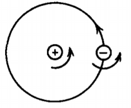
Classical atomic models describe an atom as orbiting electrons about a positively charged nucleus, as in Figure 5-13.

Figure 5-13 Atomic currents arise from orbiting electrons in addition to the spin contributions from the electron and nucleus

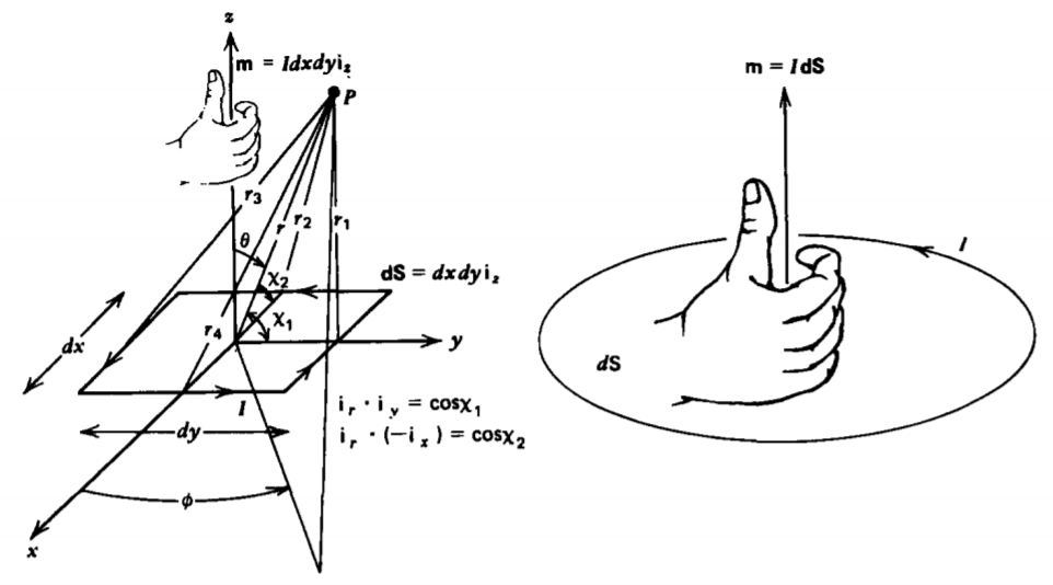
The nucleus and electron can also be imagined to be spinning. The simplest model for these atomic currents is analogous to the electric dipole and consists of a small current loop of area dS carrying a current I, as in Figure 5-14. Because atomic dimensions are so small, we are only interested in the magnetic field far from this magnetic dipole. Then the shape of the loop is not important, thus for simplicity we take it to be rectangular

The vector potential for this loop is then

\[\textbf{A} = \frac{\mu_{0}I}{4 \pi} \bigg[ dx \bigg(\frac{1}{r_{3}} - \frac{1}{r_{1}} \bigg) \textbf{i}_{x} + dy \bigg( \frac{1}{r_{4}} - \frac{1}{r_{2}} \bigg) \textbf{i}_{y} \bigg] \]

where we assume that the distance from any point on each side of the loop to the field point P is approximately constant.

Figure 5-14 A magnetic dipole consists of a small circulating current loop. The magnetic moment is in the direction normal to the loop by the right-hand rule.

Using the law of cosines, these distances are related as

\[r_{1}^{2} = r^{2} + \bigg( \frac{dy}{2} \bigg) ^{2} - r dy \cos \chi_{1}; \: \: \: \: r_{2}^{2} = r^{2} + \bigg( \frac{dx}{2} \bigg)^{2} - r dx \cos \chi_{2} \\ r_{3}^{2} = r^{2} + \bigg( \frac{dy}{2} \bigg)^{2} + r dy \cos \chi_{1}, \: \: \: \: r_{4}^{2} = r^{2} + \bigg( \frac{dx}{2} \bigg) ^{2} + r dx \cos \chi_{2} \]

where the angles \(\chi_{1}\) and \(\chi_{2}\) are related to the spherical coordinates from Table 1-2 as

\[\textbf{i}_{r} \cdot \textbf{i}_{y} = \cos \chi_{1} = \sin \theta \sin \phi \\ - \textbf{i}_{r} \cdot \textbf{i}_{x} = \cos \chi_{2} = - \sin \theta \cos \phi \]

In the far field limit (1) becomes

\[\lim_{r >> dx \\ d >> dy} \textbf{A} = \frac{\mu_{0}I}{4 \pi} \bigg[ \frac{dx}{r} \bigg( \frac{1}{\bigg[ 1 + \frac{dy}{dr} \bigg( \frac{dy}{2r} + 2 \cos \chi_{1} \bigg) \bigg] ^{1/2}} \\ - \frac{1}{\bigg[1 + \frac{dy}{2r} \bigg( \frac{dy}{2r} - 2 \cos \chi_{1} \bigg) \bigg]^{1/2} } \bigg) \\ + \frac{dy}{r} \bigg( \frac{1}{\bigg[ 1 + \frac{dx}{2r} \bigg( \frac{dx}{2r} + 2 \cos \chi_{2} \bigg) \bigg]^{1/2}} - \frac{1}{\bigg[ 1 + \frac{dx}{2r} \bigg( \frac{dx}{2r} -2 \cos \chi_{2} \bigg) \bigg]^{1/2}} \bigg) \bigg] \approx \frac{- \mu_{0}I}{4 \pi r^{2}} dx dy [ \cos \chi_{1} \textbf{i}_{x} + \cos\chi_{2} \textbf{i}_{y}] \]

Using (3), (4) further reduces to

\[\textbf{A} = \frac{\mu_{0}I d \textrm{S}}{4 \pi r^{2}} \sin \theta [ - sin \phi \textbf{i}_{x} + \cos \phi \textbf{i}_{y} ] \\ = \frac{\mu_{0}I d \textrm{S}}{4 \pi r^{2}} \sin \theta \textbf{i}_{\phi} \]

where we again used Table 1-2 to write the bracketed Cartesian unit vector term as \(\textbf{i}_{\phi}\). The magnetic dipole moment m is defined as the vector in the direction perpendicular to the loop (in this case \(\textbf{i}_{z}\)) by the right-hand rule with magnitude equal to the product of the current and loop area:

\[\textbf{m} = I \: d \textrm{S} \textbf{i}_{z} = I \: \textbf{dS} \]

Then the vector potential can be more generally written as

\[\textbf{A} = \frac{\mu_{0}m}{4 \pi r^{2}} \sin \theta \textbf{i}_{\phi} = \frac{\mu_{0} \textbf{m}}{4 \pi r^{2}} \times \textbf{i}_{r} \]

with associated magnetic field

\[\textbf{B} = \nabla \times \textbf{A} = \frac{1}{r \sin \theta} \frac{\partial}{\partial \theta} (A_{\phi} \sin \theta) \textbf{i}_{r} - \frac{1}{r} \frac{\partial}{\partial r} (r A_{\phi}) \textbf{i}_{\phi} \\ = \frac{\mu_{0} m}{4 \pi r^{3}} [2 \cos \theta \textbf{i}_{r} + \sin \theta \textbf{i}_{\theta}] \]

This field is identical in form to the electric dipole field of Section 3-1-1 if we replace \(p/\varepsilon_{0}\) by \(\mu_{0} m\).

5-5-2 Magnetization Currents

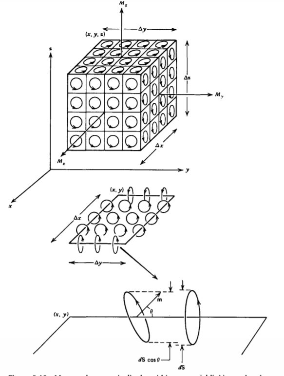
Ampere modeled magnetic materials as having the volume filled with such infinitesimal circulating current loops with number density N, as illustrated in Figure 5-15. The magnetization vector M is then defined as the magnetic dipole density:

\[\textbf{M} = N \textbf{m} = NI \textbf{dS} \textrm{amp/m} \]

For the differential sized contour in the xy plane shown in Figure 5-15, only those dipoles with moments in the x or y directions (thus z components of currents) will give rise to currents crossing perpendicularly through the surface bounded by the contour. Those dipoles completely within the contour give no net current as the current passes through the contour twice, once in the positive z direction and on its return in the negative z direction. Only those dipoles on either side of the edges-so that the current only passes through the contour once, with the return outside the contour-give a net current through the loop.

Because the length of the contour sides \(\Delta x\) and \(\Delta y\) are of differential size, we assume that the dipoles along each edge do not change magnitude or direction. Then the net total current linked by the contour near each side is equal to the product of the current per dipole I and the number of dipoles that just pass through the contour once. If the normal vector to the dipole loop (in the direction of m) makes an angle \(\theta\) with respect to the direction of the contour side at position x, the net current linked along the line at x is

\[- IN d \textrm{S} \Delta y \cos \theta \big|_{x} = -M_{y}(x) \Delta y \]

The minus sign arises because the current within the contour adjacent to the line at coordinate x flows in the - z direction.

Figure 5-15 Many such magnetic dipoles within a material linking a closed contour gives rise to an effective magnetization current that is also a source of the magnetic field.

Similarly, near the edge at coordinate \(x + \Delta x \), the net current linked perpendicular to the contour is

\[IN \: d \textrm{S} \Delta y \cos \theta \big|_{x + \Delta x} = M_{y} (x + \Delta x) \Delta y \]

Along the edges at y and \(y + \Delta y\), the current contributions are

\[IN \: d \textrm{S} \Delta x \: \cos \theta \big|_{y} = M_{x}(y) \Delta x \\ = - IN \: d \textrm{S} \: \Delta x \cos \theta \big|_{y + \Delta y} = - M_{x}(y + \Delta y) \Delta x \]

The total current in the z direction linked by this contour is thus the sum of contributions in (10)-(12):

\[I_{z \textrm{tot}} = \Delta x \Delta \bigg( \frac{M_{y} (x + \Delta x) - M_{y}(x)}{\Delta x} - \frac{M_{x}(y + \Delta y) - M_{x}(y)}{\Delta y}\bigg) \]

If the magnetization is uniform, the net total current is zero as the current passing through the loop at one side is canceled by the current flowing in the opposite direction at the other side. Only if the magnetization changes with position can there be a net current through the loop's surface. This can be accomplished if either the current per dipole, area per dipole, density of dipoles, of angle of orientation of the dipoles is a function of position.

In the limit as \(\Delta x\) and\(\Delta y\) become small, terms on the right-hand side in (13) define partial derivatives so that the current per unit area in the z direction is

\[\lim_{\Delta x \rightarrow 0 \\ \Delta y \rightarrow 0} J_{z} = \frac{I_{z \textrm{ tot}}}{\Delta x \Delta y} = \bigg( \frac{\partial M_{y}}{\partial x} - \frac{\partial M_{x}}{\partial y} \bigg) = ( \nabla \times \textbf{M})_{z} \]

which we recognize as the z component of the curl of the magnetization. If we had orientated our loop in the xz or yz planes, the current density components would similarly obey the relations

\[J_{y} = \bigg( \frac{\partial M_{x}}{\partial z} - \frac{\partial M_{z}}{\partial x} \bigg) = (\nabla \times \textbf{M})_{y} \\ J_{x} = \bigg( \frac{\partial M_{z}}{\partial y} - \frac{\partial M_{y}}{\partial z} \bigg) = (\nabla \times \textbf{M})_{x} \]

so that in general 

\[ \mathbf{J}_m=\nabla \times \mathbf{M} \]

where we subscript the current density with an m to represent the magnetization current density, often called the Amperian current density.

These currents are also sources of the magnetic field and can be used in Ampere's law as

\[\nabla \times \frac{\textbf{B}}{\mu_{0}} = \textbf{J}_{m} + \textbf{J}_{f} = \textbf{J}_{f} + \nabla \times \textbf{M} \]

where \(\textbf{J}_{f}\) is the free current due to the motion of free charges as contrasted to the magnetization current \(\textbf{J}_{m}\), which is due to the motion of bound charges in materials.

As we can only impose free currents, it is convenient to define the vector H as the magnetic field intensity to be distinguished from B, which we will now call the magnetic flux density:

\[\textbf{H} = \frac{\textbf{B}}{\mu_{0}} - \textbf{M} \Rightarrow \textbf{B} = \mu_{0} (\textbf{H} + \textbf{M}) \]

Then (17) can be recast as

\[\nabla \times \bigg( \frac{\textbf{B}}{\mu_{0}} - \textbf{M} \bigg) = \nabla \times \textbf{H} = \textbf{J}_{f} \]

The divergence and flux relations of Section 5-3-1 are unchanged and are in terms of the magnetic flux density B. In free space, where M = 0, the relation of (19) between B and H reduces to

\[\textbf{B} = \mu_{0} \textbf{H} \]

This is analogous to the development of the polarization with the relationships of D, E, and P. Note that in (18), the constant parameter \(\mu_{0}\) multiplies both H and M, unlike the permittivity \(\mu_{0}\) which only multiplies E.

Equation (19) can be put into an equivalent integral form using Stokes' theorem:

\[\int_{S} (\nabla \times \textbf{H}) \cdot \textbf{dS} = \oint_{L} \textbf{H} \cdot \textbf{dl} = \int_{S} \textbf{J}_{f} \cdot \textbf{dS} \]

The free current density \(\textbf{J}_{f}\) is the source of the H field, the magnetization current density \(\textbf{J}_{m}\). is the source of the M field, while the total current, \(\textbf{J}_{f} + \textbf{J}_{m}\), is the source of the B field.

5-5-3 Magnetic Materials

There are direct analogies between the polarization processes found in dielectrics and magnetic effects. The constitutive law relating the magnetization M to an applied magnetic field H is found by applying the Lorentz force to our atomic models.

(a) Diamagnetism

The orbiting electrons as atomic current loops is analogous to electronic polarization, with the current in the direction opposite to their velocity. If the electron (e = 1.6 x 10^-9 coul) rotates at angular speed \(\omega\) at radius R, as in Figure 5-16, the current and dipole moment are

\[I = \frac{e \omega}{2 \pi}, \: \: \: \: m = I \pi R^{2} = \frac{e \omega}{2} R^{2} \]

Figure 5-16 The orbiting electron has its magnetic moment m in the direction opposite to its angular momentum L because the current is opposite to the electron's velocity.

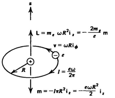
Note that the angular momentum L and magnetic moment m are oppositely directed and are related as

\[\textbf{L} = m_{e} R \textbf{i}_{r} \times \textbf{v} = m_{e} \omega R^{2} \textbf{i}_{z} = - \frac{2m_{e}}{e} \textbf{m} \]

where m_e = 9.1 x 10^-31 kg is the electron mass.

Since quantum theory requires the angular momentum to be quantized in units of \(h/2 \pi\), where Planck's constant is \(h = 6.62 \times 10{-34}\) joule-sec, the smallest unit of magnetic moment, known as the Bohr magneton, is

\[m_{B} = \frac{eh}{4 \pi m_{e}} \approx 9.3 \times 10^{-24} \textrm{amp m}^{2} \]

Within a homogeneous material these dipoles are randomly distributed so that for every electron orbiting in one direction, another electron nearby is orbiting in the opposite direction so that in the absence of an applied magnetic field there is no net magnetization.

The Coulombic attractive force on the orbiting electron towards the nucleus with atomic number Z is balanced by the centrifugal force:

\[m_{e} \omega^{2} R = \frac{Z e^{2}}{4 \pi \varepsilon_{0}R^{2}} \]

Since the left-hand side is just proportional to the square of the quantized angular momentum, the orbit radius R is also quantized for which the smallest value is

\[R = \frac{4 \pi \varepsilon_{0}}{m_{e}Ze^{2}} \bigg( \frac{h}{2 \pi} \bigg)^{2} \approx \frac{5 \times 10^{-11}}{Z} \textrm{m} \]

with resulting angular speed

\[\omega = \frac{Z^{2}e^{4}m_{e}}{(4 \pi \varepsilon_{0})^{2}(h/2 \pi)^{3}} \approx 1.3 \times 10^{16}Z^{2} \]

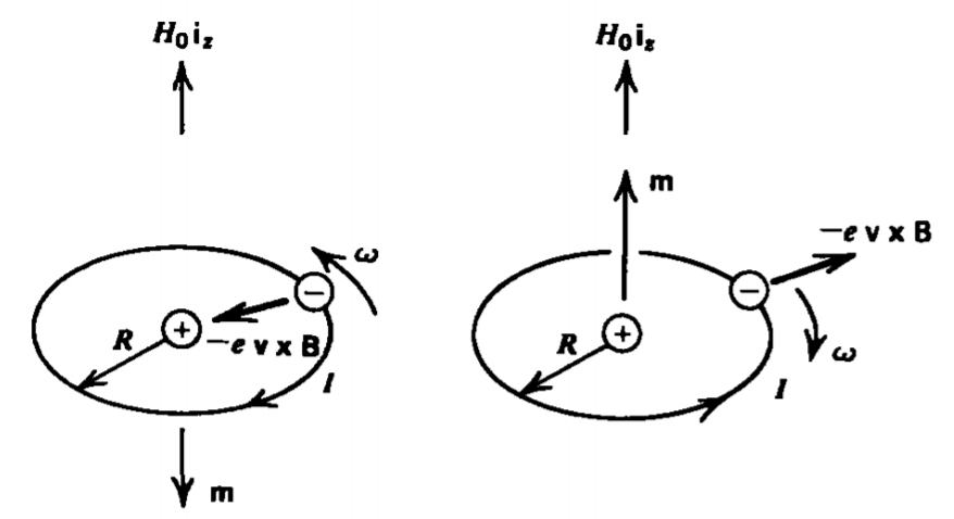
When a magnetic field \(H_{0}\textbf{i}_{z}\) is applied, as in Figure 5-17, electron loops with magnetic moment opposite to the field feel an additional radial force inwards, while loops with colinear moment and field feel a radial force outwards. Since the orbital radius R cannot change because it is quantized, this magnetic force results in a change of orbital speed \(\Delta \omega\):

\[m_{e}(\omega + \Delta \omega_{1})^{2} R = e \bigg( \frac{Ze}{4 \pi \varepsilon_{0}R^{2}} + (\omega + \Delta \omega_{1}) R \mu_{0}H_{0} \bigg) \\ m_{e}(\omega + \Delta \omega_{2})^{2} R= e \bigg( \frac{Ze}{4 \pi \varepsilon_{0}R^{2}} - (\omega + \Delta \omega_{2}) R \mu_{0} H_{0} \bigg) \]

where the first electron speeds up while the second one slows down.

Because the change in speed \(\Delta \omega\) is much less than the natural speed \(\omega\), we solve (28) approximately as

\[\Delta \omega_{1} = \frac{e \omega \mu_{0} H_{0}}{2 m_{e} \omega - e \mu_{0} H_{0}} \\ \Delta \omega_{2} = \frac{- e \omega \mu_{0} H_{0}}{2 m_{e} \omega + e \mu_{0} H_{0}} \]

where we neglect quantities of order \((\Delta \omega)^{2}\). However, even with very high magnetic field strengths of \(H_{0} 10^{6}\) amp/m we see that usually

\[e \mu_{0} H_{0} << 2 m_{e} \omega_{0} \\ (1.6 \times 10^{-19})(4 \pi 10^{-7}) 10^{6} << 2(9.1 \times 10^{-31})(1.3 \times 10^{16}) \]

so that (29) further reduces to

\[\Delta \omega_{1} \approx - \Delta \omega_{2} \approx \frac{e \mu_{0}H_{0}}{2 m_{e}} \approx 1.1 \times 10^{5} H_{0} \]

The net magnetic moment for this pair of loops,

\[m = \frac{eR^{2}}{2} (\omega_{2} - \omega_{1}) = -eR^{2} \Delta \omega_{1} = \frac{- e^{2} \mu_{0}R^{2}}{2 m_{e}} H_{0} \]

is opposite in direction to the applied magnetic field.

Figure 5-17 Diamagnetic effects, although usually small, arise in all materials because dipoles with moments parallel to the magnetic field have an increase in the orbiting electron speed while those dipoles with moments opposite to the field have a decrease in speed. The loop radius remains constant because it is quantized.

If we have N such loop pairs per unit volume, the magnetization field is

\[\textbf{M} = N \textbf{m} = - \frac{Ne^{2} \mu_{0} R^{2}}{2m_{e}} H_{0}\textbf{i}_{z} \]

which is also oppositely directed to the applied magnetic field

Since the magnetization is linearly related to the field, we define the magnetic susceptibility \(\chi_{m}\) as

\[\textbf{M} = \chi_{m} \textbf{H}, \: \: \: \: \chi_{m} = - \frac{Ne^{2}\mu_{0}R^{2}}{2 m_{e}} \]

where \(\chi_{m}\) is negative. The magnetic flux density is then

\[\textbf{B} = \mu_{0}(\textbf{H} + \textbf{M}) = \mu_{0}(1 + \chi_{m}) \textbf{H} = \mu_{0} \mu_{r} \textbf{H} = \mu \textbf{H} \]

where \(\mu_{r} = 1 + \chi_{m}\) is called the relative permeability and \(\mu\) is the permeability. In free space \(\chi_{m} = 0 \) so that \(\mu_{r} = 1\) and \(\mu = \mu_{0}\). The last relation in (35) is usually convenient to use, as all the results in free space are still correct within linear permeable material if we replace \(\mu_{0}\) by \(\mu\). In diamagnetic materials, where the susceptibility is negative, we have that \(\mu_{r} < 1, \: \mu < \mu_{0}\). However, substituting in our typical values

\[\chi_{m} = - \frac{Ne^{2}\mu_{0}R^{2}}{2 m.} \approx \frac{4.4 \times 10^{-35}}{Z^{2}}N \]

we see that even with \(N \approx 10^{30}\) atoms/m³ , \(\chi_{m}\) is much less than unity so that diamagnetic effects are very small.

(b) Paramagnetism

As for orientation polarization, an applied magnetic field exerts a torque on each dipole tending to align its moment with the field, as illustrated for the rectangular magnetic dipole with moment at an angle \(\theta\) to a uniform magnetic field B in Figure 5-18a. The force on each leg is

\[\textbf{df}_{1} = - \textbf{df}_{2} = I \Delta x \: \Delta x \: \textbf{i}_{x} \times \textbf{B} = I \: \Delta x[B_{y} \textbf{i}_{z} - B_{z} \textbf{i}_{y}] \\ \textbf{df}_{3} = - \textbf{df}_{4} = I \: \Delta y \: \textbf{i}_{y} \times \textbf{B} = I \: \Delta y (-B_{x} \textbf{i}_{z} + B_{z} \textbf{i}_{x}) \]

In a uniform magnetic field, the forces on opposite legs are equal in magnitude but opposite in direction so that the net

Figure 5-18 (a) A torque is exerted on a magnetic dipole with moment at an angle \(\theta\) to an applied magnetic field. (b) From Boltzmann statistics, thermal agitation opposes the alignment of magnetic dipoles. All the dipoles at an angle \(\theta\), together have a net magnetization in the direction of the applied field.

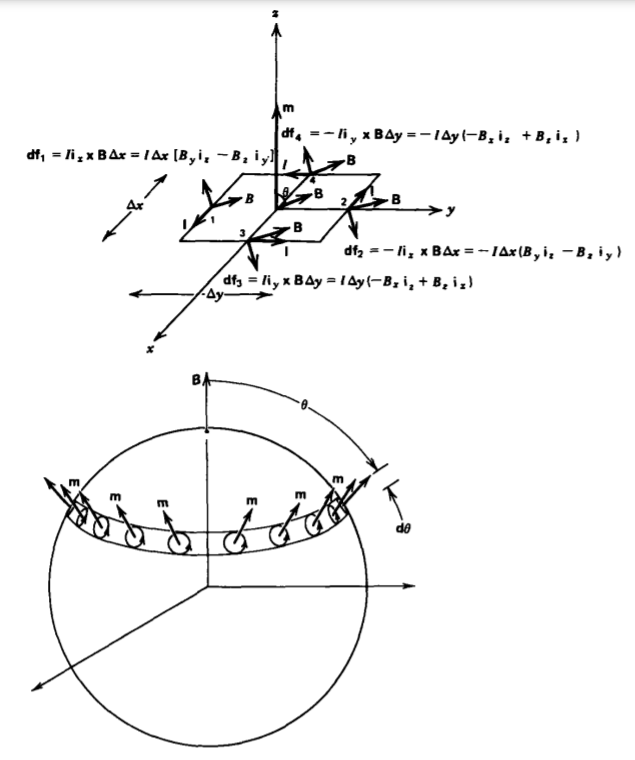
force on the loop is zero. However, there is a torque:

\[\textbf{T} = \sum_{n=1}^{4} \textbf{r} \times \textbf{df}_{n} \\ = \frac{\Delta y}{2} (- \textbf{i}_{y} \times \textbf{df}_{1} + \textbf{i}_{y} \times \textbf{df}_{2}) + \frac{\Delta x}{2} (\textbf{i}_{x} \times \textbf{df}_{3} - \textbf{i}_{x} \times \textbf{df}_{4}) \\ = I \Delta x \: \Delta y (B_{x}i_{y} - B_{y}\textbf{i}_{x}) = \textbf{m} \times \textbf{B} \]

The incremental amount of work necessary to turn the dipole by a small angle \(d \theta\) is

\[dW = T \: d \theta = m \mu_{0} H_{0} \sin \theta d \theta \]

so that the total amount of work necessary to turn the dipole from \(\theta = 0\) to any value of \(\theta\) is

\[W = \int_{0}^{\theta} T \: d \theta = - m \mu_{0} H_{0} \cos \theta \big|_{0}^{\theta} = m \mu_{0} H_{0} (1-\cos \theta) \]

This work is stored as potential energy, for if the dipole is released it will try to orient itself with its moment parallel to the field. Thermal agitation opposes this alignment where Boltzmann statistics describes the number density of dipoles having energy W as

\[n = n_{1} e^{-W/kT} = n_{1} e^{-m \mu_{0} H_{0} (1-\cos \theta)/kT} = n_{0} e^{m \mu_{0} H_{0} \cos \theta/ kT} \]

where we lump the constant energy contribution in (40) within the amplitude \(n_{0}\), which is found by specifying the average number density of dipoles N within a sphere of radius R:

\[N = \frac{1}{\frac{4}{3} \pi R^{3}} \int_{\theta = 0}^{\pi} \int_{\phi = 0}^{2 \pi} \int_{r = 0 }^{R} n_{0} e^{a \cos \theta} r^{2} \sin \theta dr \: d \theta \: d \phi \\ = \frac{n_{0}}{2} \int_{\theta = 0}^{\pi} \sin \theta e^{a \cos theta} d \theta \]

where we let

\[a = m \mu_{0} H_{0}/kT \]

With the change of variable

\[u = a \cos \theta, \: \: \: \: du = -a \sin \theta \: d \theta \]

the integration in (42) becomes

\[N = \frac{-n_{0}}{2a} \int_{a}^{-a} e^{u} du = \frac{n_{0}}{a} \sinh a \]

so that (41) becomes

\[n = \frac{N_{a}}{\sinh a} e^{a \cos \theta} \]

From Figure 5-18b we see that all the dipoles in the shell over the interval \(\theta\) to \(\theta + d \theta\) contribute to a net magnetization. which is in the direction of the applied magnetic field:

\[dM = \frac{mn}{\frac{4}{3} \pi R^{3}} \cos \theta r^{2} \sin \theta \: dr \: d \theta \: d \phi \]

so that the total magnetization due to all the dipoles within the sphere is

\[M = \frac{maN}{2 \sinh a} \int_{\theta = 0}^{\pi} \sin \theta \cos \theta e^{a \cos \theta} d \theta \]

Again using the change of variable in (44), (48) integrates to

\[M = \frac{-mN}{2a \sinh a} \int_{a}^{-a} u e^{u} du \\ = \frac{-m N}{2a \sinh a} e^{u} (u-1) \big|_{a}^{a} \\ = \frac{-mN}{2a \sinh a} [e^{-a} (-a -1) - e^{a} (a-1)] \\ = \frac{-mN}{a \sinh a} [-a \cosh a + \sinh a] \\ = mN[\coth a -1/a] \]

which is known as the Langevin equation and is plotted as a function of reciprocal temperature in Figure 5-19. At low temperatures (high a) the magnetization saturates at M = mN as all the dipoles have their moments aligned with the field. At room temperature, a is typically very small. Using the parameters in (26) and (27) in a strong magnetic field of \(H_{0} = 10^{6}\) amps/m, a is much less than unity:

\[a = \frac{m \mu_{0}H_{0}}{kT} = \frac{e \omega}{2} R^{2} \frac{\mu_{0}H_{0}}{kT} \approx 8 \times 10^{-4} \]

Figure 5-19 The Langevin equation describes the net magnetization. At low temperatures (high a) all the dipoles align with the field causing saturation. At high temperatures (a << 1) the magnetization increases linearly with field.

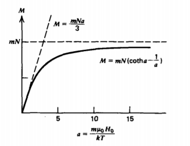
In this limit, Langevin's equation simplifies to

\[\lim_{a << 1}M \approx mN \bigg[ \frac{1 + a^{2}/2}{a + a^{3}/6} - \frac{1}{a} \bigg] \\ \approx mN \bigg( \frac{(1 + a^{2}/2)(1-a^{3}/6)}{a} = \frac{1}{a} \bigg] \\ \approx \frac{mNa}{3} \approx \frac{\mu_{0}m^{2}N}{3kT}H_{0} \]

In this limit the magnetic susceptibility \(\chi_{m}\) is positive:

\[\textbf{M} = \chi_{m}\textbf{H}, \: \: \: \chi_{m} = \frac{\mu_{0}m^{2}N}{3 kT} \]

but even with \(N \approx 10^{30}\) atoms/m³ , it is still very small:

\[\chi_{m} \approx 7 \times 10^{-4} \]

(c) Ferromagnetism

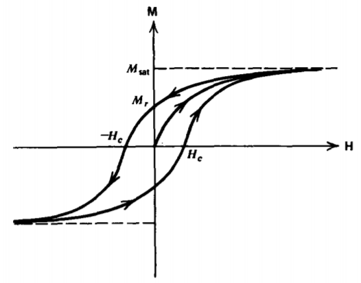
As for ferroelectrics (see Section 3-1-5), sufficiently high coupling between adjacent magnetic dipoles in some iron alloys causes them to spontaneously align even in the absence of an applied magnetic field. Each of these microscopic domains act like a permanent magnet, but they are randomly distributed throughout the material so that the macroscopic magnetization is zero. When a magnetic field is applied, the dipoles tend to align with the field so that domains with a magnetization along the field grow at the expense of nonaligned domains.

The friction-like behavior of domain wall motion is a lossy process so that the magnetization varies with the magnetic field in a nonlinear way, as described by the hysteresis loop in Figure 5-20. A strong field aligns all the domains to saturation. Upon decreasing H, the magnetization lags behind so that a remanent magnetization M_r exists even with zero field. In this condition we have a permanent magnet. To bring the magnetization to zero requires a negative coercive field -H_c.

Although nonlinear, the main engineering importance of ferromagnetic materials is that the relative permeability \(\mu_{r}\) is often in the thousands:

\[\mu = \mu_{r} \mu_{0} = \textbf{B}/\textbf{H} \]

This value is often so high that in engineering applications we idealize it to be infinity. In this limit

\[\lim_{\mu \rightarrow \infty} \textbf{B} = \mu \textbf{H} \Rightarrow \textbf{H} = 0, \: \: \: \: \textbf{B} \: \textrm{ finite} \]

the H field becomes zero to keep the B field finite.

Figure 5-20 Ferromagnetic materials exhibit hysteresis where the magnetization saturates at high field strengths and retains a net remanent magnetization M_r even when H is zero. A coercive field -H_c is required to bring the magnetization back to zero.

Example 5-1: Infinite Line Current Within a Magnetically Permeable Cylinder

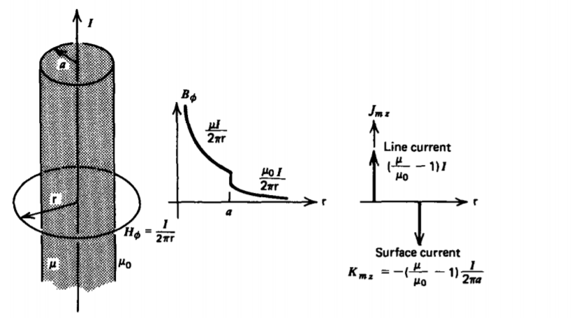
A line current I of infinite extent is within a cylinder of radius a that has permeability \(\mu\), as in Figure 5-21. The cylinder is surrounded by free space. What are the B, H, and M fields everywhere? What is the magnetization current?

Figure 5-21 A free line current of infinite extent placed within a permeable cylinder gives rise to a line magnetization current along the axis and an oppositely directed surface magnetization current on the cylinder surface.

Solution

Pick a circular contour of radius r around the current. Using the integral form of Ampere's law, (21), the H field is of the same form whether inside or outside the cylinder:

\(\oint_{L} \textbf{H} \cdot \textbf{dl} = H_{\phi} 2 \pi \textrm{r} = I \Rightarrow H_{\phi} = \frac{I}{2 \pi \textrm{r}} \nonumber \)

The magnetic flux density differs in each region because the permeability differs:

\(B_{\phi} = \left \{ \begin{matrix} \mu H_{\phi} = \frac{\mu I}{2 \pi \textrm{r}}, & 0 < \textrm{r} < a \\ \mu_{0} H_{\phi} = \frac{\mu_{0}I}{2 \pi \textrm{r}}, & \textrm{r} > a \end{matrix} \right. \nonumber \)

The magnetization is obtained from the relation

\(\textbf{M} = \frac{\textbf{B}}{\mu_{0}} - \textbf{H} \nonumber \)

as

\[M_{\phi} = \left \{ \begin{matrix} \bigg(\frac{\mu}{\mu_{0}} - 1 \bigg) H_{\phi} = \frac{\mu - \mu_{0}}{\mu_{0}} \frac{I}{2 \pi \textrm{r}}, & 0 < \textrm{r} < a \\ 0, & \textrm{r} > a \end{matrix} \right. \nonumber \]

The volume magnetization current can be found using (16):

\[\textbf{J}_{m} = \nabla \times \textbf{M} = - \frac{\partial M_{\phi}}{\partial z} \textbf{i}_{\textrm{r}} + \frac{1}{r} \frac{\partial}{\partial textrm{r}}( \textrm{r} M_{\phi}) \textbf{i}_{z} = 0, \: \: \: \: 0 < \textrm{r} < a \nonumber \]

There is no bulk magnetization current because there are no bulk free currents. However, there is a line magnetization current at r =0 and a surface magnetization current at r = a. They are easily found using the integral form of (16) from Stokes' theorem:

\[\int_{S} \nabla \times \textbf{M} \cdot \textbf{dS} = \oint_{L} \textbf{M} \cdot \textbf{dl} = \int_{S} \textbf{J}_{m} \cdot \textbf{dS} \nonumber \]

Pick a cortour around the center of the cylinder with r < a

\[M_{\phi} 2 \pi \textrm{r} = \bigg( \frac{\mu - \mu_{0}}{\mu_{0}} \bigg) I = I_{m} \nonumber \]

where \(I_{m}\) is the magnetization line current. The result remains unchanged for any radius r<a as no more current is enclosed since \(\textbf{J}_{m} = 0 \) for 0 < r < a. As soon as r > a, \(M_{\phi}\) becomes zero so that the total magnetization current becomes zero. Therefore, at r = a a surface magnetization current must flow whose total current is equal in magnitude but opposite in sign to the line magnetization current:

\[K_{zm} = \frac{-I_{m}}{2 \pi a} = - \frac{\mu - \mu_{0})I}{\mu_{0} 2 \pi a} \nonumber \]