5.6: Boundary Conditions

At interfacial boundaries separating materials of differing properties, the magnetic fields on either side of the boundary must obey certain conditions. The procedure is to use the integral form of the field laws for differential sized contours, surfaces, and volumes in the same way as was performed for electric fields in Section 3-3.

To summarize our development thus far, the field laws for magnetic fields in differential and integral form are

\[\nabla \times \textbf{H} = \textbf{J}_{f}, \: \: \: \: \oint_{L} \textbf{H} \cdot \textbf{dl} = \int_{S} \textbf{J}_{f} \cdot \textbf{dS} \]

\[\nabla \times \textbf{M} = \textbf{J}_{m}, \: \: \: \: \oint_{L} \textbf{M} \cdot \textbf{dl} = \int_{S} \textbf{J}_{m} \cdot \textbf{dS} \]

\[\nabla \cdot \textbf{B} = 0, \: \: \: \: \oint_{S} \textbf{B} \cdot \textbf{dS} = 0 \]

5-6-1 Tangential Component of H

We apply Ampere's circuital law of (1) to the contour of differential size enclosing the interface, as shown in Figure 5-22a. Because the interface is assumed to be infinitely thin, the short sides labelled c and d are of zero length and so offer

Figure 5-22 (a) The tangential component of H can be discontinuous in a free surface current across a boundary. (b) The normal component of B is always continu­ous across an interface.

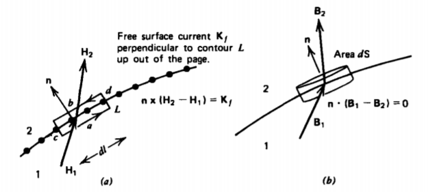
no contribution to the line integral. The remaining two sides yield

\[\oint_{L} \textbf{H} \cdot \textbf{dl} = (H_{1t} - H_{2t}) dl = K_{fn} dl \]

where \(K_{fn}\). is the component of free surface current perpendicular to the contour by the right-hand rule in this case up out of the page. Thus, the tangential component of magnetic field can be discontinuous by a free surface current,

\[(H_{1t}-H_{2t}) = K_{fn} \Rightarrow \textbf{n} \times (\textbf{H}_{2} - \textbf{H}_{1}) = \textbf{K}_{f} \]

where the unit normal points from region 1 towards region 2. If there is no surface current, the tangential component of H is continuous.

5-6-2 Tangential Component of M

Equation (2) is of the same form as (6) so we may use the results of (5) replacing H by M and K_f by K_m the surface magnetization current:

\[(M_{1t} - M_{2t}) = K_{mn}, \: \: \: \: \textbf{n} \times (\textbf{M}_{2} - \textbf{M}_{1}) = \textbf{K}_{m} \]

This boundary condition confirms the result for surface magnetization current found in Example 5-1.

5-6-3 Normal Component of B

Figure 5-22b shows a small volume whose upper and lower surfaces are parallel and are on either side of the interface. The short cylindrical side, being of zero length, offers no contribution to (3), which thus reduces to

\[\oint_{S} \textbf{B} \cdot \textbf{dS} = (B_{2n} - B_{1n}) d \textrm{S} =0 \]

yielding the boundary condition that the component of B normal to an interface of discontinuity is always continuous:

\[B_{1n} - B_{2n} = 0 \Rightarrow \textbf{n} \cdot (\textbf{B}_{1} - \textbf{B}_{2}) = 0 \]

Example 5-2: Magnetic Slab Within A Uniform Magnetic Field

A slab of infinite extent in the x and y directions is placed within a uniform magnetic field \(H_{0}\textbf{i}_{z}\) as shown in Figure 5-23.

Figure 5-23 A (a) permanently magnetized or (b) linear magnetizable material is placed within a uniform magnetic field.

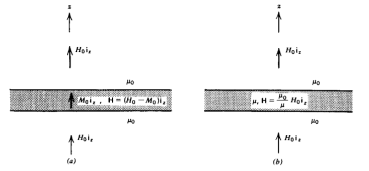
Find the H field within the slab when it is

(a) permanently magnetized with magnetization \(M_{0}\textbf{i}_{z}\)

(b) a linear permeable material with permeability \(\mu\).

Solution

For both cases, (8) requires that the B field across the boundaries be continuous as it is normally incident.

(a) For the permanently magnetized slab, this requires that

\(\mu_{0} H_{0} = \mu_{0} (H + M_{0}) \Rightarrow H = H_{0} - M_{0}\)

Note that when there is no externally applied field (\(H_{0}\) = 0), the resulting field within the slab is oppositely directed to the magnetization so that B = 0.

(b) For a linear permeable medium (8) requires

\(\mu_{0}H_{0} = \mu H \Rightarrow H = \frac{\mu_{0}}{\mu} H_{0}\)

For \(\mu > \mu_{0}\) the internal magnetic field is reduced. If \(H_{0}\) is set to zero, the magnetic field within the slab is also zero.