5.7: Magnetic Field Boundary Value Problems

5-7-1 The Method of Images

A line current I of infinite extent in the z direction is a distance d above a plane that is either perfectly conducting or infinitely permeable, as shown in Figure 5-24. For both cases

Figure 5-24 (a) A line current above a perfect conductor induces an oppositely directed surface current that is equivalent to a symmetrically located image line current. (b) The field due to a line current above an infinitely permeable medium is the same as if the medium were replaced by an image current now in the same direction as the original line current.

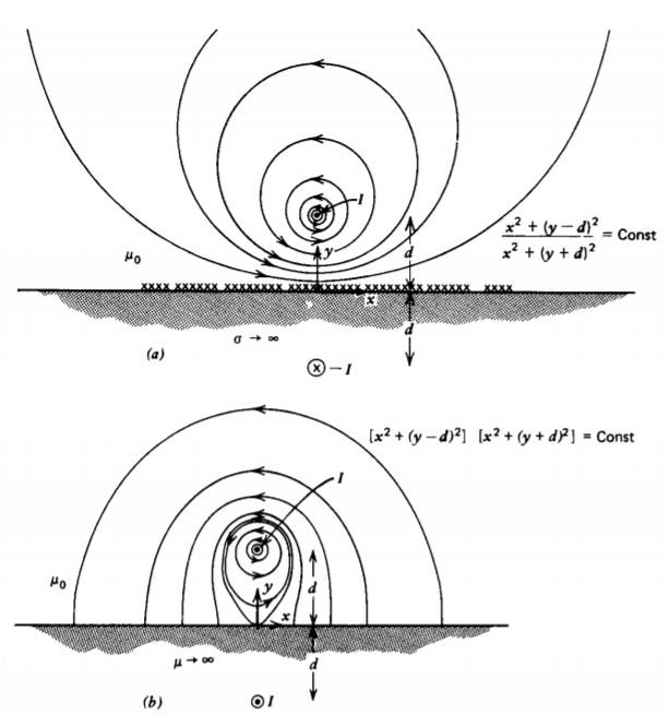
the H field within the material must be zero but the boundary conditions at the interface are different. In the perfect conductor both B and H must be zero, so that at the interface the normal component of B and thus H must be continuous and thus zero. The tangential component of H is discontinuous in a surface current.

In the infinitely permeable material H is zero but B is finite. No surface current can flow because the material is not a conductor, so the tangential component of H is continuous and thus zero. The B field must be normally incident.

Both sets of boundary conditions can be met by placing an image current I at y = -d flowing in the opposite direction for the conductor and in the same direction for the permeable material.

Using the upper sign for the conductor and the lower sign for the infinitely permeable material, the vector potential due to both currents is found by superposing the vector potential found in Section 5-4-3a, Eq. (18), for each infinitely long line current:

\[A_{z} = \frac{-\mu_{0}I}{2 \pi} (\ln [ x^{2} + (y-d)^{2}]^{1/2} \mp \ln[x^{2} + (y + d)^{2}]^{1/2}) \\ = \frac{- \mu_{0}I}{4 \pi} (\ln [x^{2} + (y-d)^{2}] \mp \ln [x^{2} + (y + d)^{2}]) \]

with resultant magnetic field

\[\textbf{H} = \frac{1}{\mu_{0}} \nabla \times \textbf{A} = \frac{1}{\mu_{0}} \bigg(\textbf{i}_{x} \frac{\partial A_{z}}{\partial y} - \textbf{i}_{y} \frac{\partial A_{z}}{\partial x} \bigg) = \frac{-I}{2 \pi} \left \{ \begin{matrix} \frac{(y-d) \textbf{i}_{x} - x \textbf{i}_{y}}{[x^{2} + (y-d)^{2}]} \mp \frac{(y + d) \textbf{i}_{x} - x \textbf{i}_{y}}{[x^{2} + (y + d)^{2}]} \end{matrix} \right. \]

The surface current distribution for the conducting case is given by the discontinuity in tangential H,

\[K_{z} = - H_{x} (y=0) = - \frac{Id}{\pi[d^{2} + x^{2}]} \]

which has total current

\[\] \[\begin{aligned} I_T & =\int_{-\infty}^{+\infty} K_{\mathrm{z}} d x=-\frac{I d}{\pi} \int_{-\infty}^{+\infty} \frac{d x}{\left(x^2+d^2\right)} \\ & =-\left.\frac{I d}{\pi} \frac{1}{d} \tan ^{-1} \frac{x}{d}\right|_{-\infty} ^{+\infty}=-I\end{aligned}\]

The force per unit length on the current for each case is just due to the magnetic field from its image:

\[\textbf{f} = \pm \frac{\mu_{0}I^{2}}{4 \pi d} \textbf{i}_{y} \]

being repulsive for the conductor and attractive for the permeable material.

The magnetic field lines plotted in Figure 5-24 are just lines of constant \(A_{z}\) as derived in Section 5-4-3b. Right next to the line current the self-field term dominates and the field lines are circles. The far field in Figure 5-24b, when the line and image current are in the same direction, is the same as if we had a single line current of 2I.

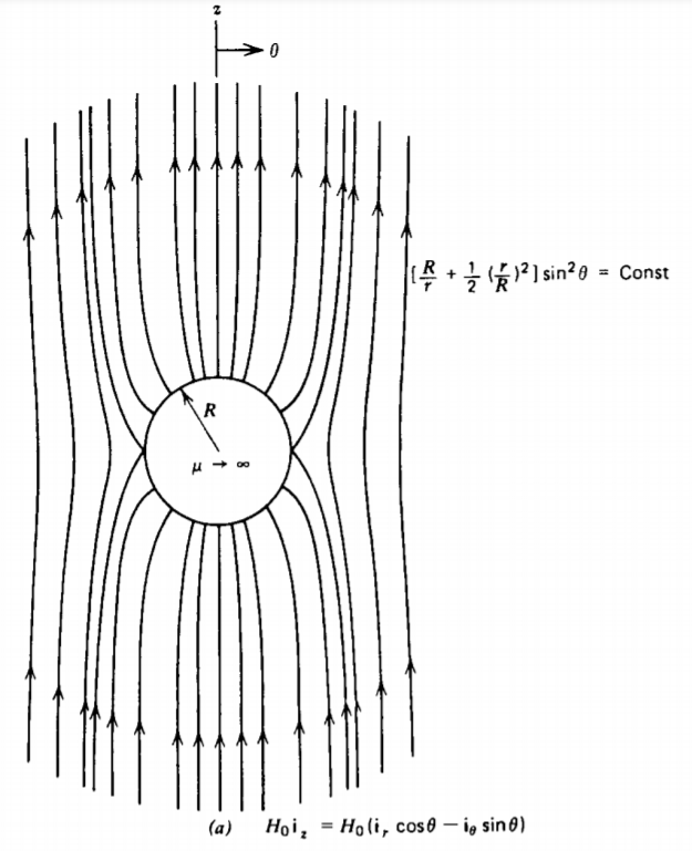
5-7-2 Sphere in a Uniform Magnetic Field

A sphere of radius R is placed within a uniform magnetic field \(H_{0} \textbf{i}_{z}\). The sphere and surrounding medium may have any of the following properties illustrated in Figure 5-25:

1. Sphere has permeability \(\mu_{2}\) and surrounding medium has permeability \(\mu_{1}\).
2. Perfectly conducting sphere in free space.
3. Uniformly magnetized sphere \(M_{2} \textbf{i}_{z}\), in a uniformly magnetized medium \(M_{1}\textbf{i}_{z}\).

For each of these three cases, there are no free currents in either region so that the governing equations in each region are

\[\nabla \cdot \textbf{B} = 0 \\ \nabla \times \textbf{H} = 0 \]

Figure 5-25 Magnetic field lines about an (a) infinitely permeable and (b) perfectly conducting sphere in a uniform magnetic field.

Figure 5-25

Because the curl of H is zero, we can define a scalar magnetic potential

\[\textbf{H} = \nabla_{\chi} \]

where we avoid the use of a negative sign as is used with the electric field since the potential \(\chi\) is only introduced as a mathematical convenience and has no physical significance. With B proportional to H or for uniform magnetization, the divergence of H is also zero so that the scalar magnetic potential obeys Laplace's equation in each region:

\[\nabla^{2}_{\chi} = 0 \]

We can then use the same techniques developed for the electric field in Section 4-4 by trying a scalar potential in each region as

\[\chi = \left \{ \begin{matrix} Ar \cos \theta, & r< R \\ (Dr + C/r^{2}) \cos \theta & r > R \end{matrix} \right. \]

The associated magnetic field is then

\[\textbf{H} = \nabla_{\chi} = \frac{\partial \chi}{\partial r} \textbf{i}_{r} + \frac{1}{r} \frac{\partial \chi}{\partial \theta} \textbf{i}_{\theta} + \frac{1}{r \sin \theta} \frac{\partial_{\chi}}{\partial \phi} \textbf{i}_{\phi} \\ = \left \{ \begin{matrix} A(\textbf{i}_{r} \cos \theta - \textbf{i}_{\theta} \sin \theta) = A \textbf{i}_{z}, & r< R \\ (D - 2C/r^{3}) \cos \theta \textbf{i}_{r} - (D + C/r^{3}) \sin \theta \textbf{i}_{\theta}, & r > R \end{matrix} \right. \]

For the three cases, the magnetic field far from the sphere must approach the uniform applied field:

\[\textbf{H}(r = \infty) = H_{0} \textbf{i}_{z} = H_{0}(\textbf{i}_{r} \cos \theta - \textbf{i}_{theta} \sin \theta) \Rightarrow D = H_{0} \]

The other constants, A and C, are found from the boundary conditions at r = R. The field within the sphere is uniform, in the same direction as the applied field. The solution outside the sphere is the imposed field plus a contribution as if there were a magnetic dipole at the center of the sphere with moment \(m_{z} = 4 \pi C\).

(i) If the sphere has a different permeability from the surrounding region, both the tangential components of H and the normal components of B are continuous across the spherical surface:

\[H_{\theta} (r = R_{+}) = H_{\theta}(r = R_{-}) \Rightarrow A = D + C/R^{3} \\ B_{r} (r = R_{+}) = B_{r} (r = R_{-}) \Rightarrow \mu_{1} H_{r}(r = R_{+}) = \mu_{2}H_{r}(r=R_{-}) \]

which yields solutions

\[A = \frac{3 \mu_{1}H_{0}}{\mu_{2} + 2 \mu_{1}}, \: \: \: \: C = - \frac{\mu_{2}-\mu_{1}}{\mu_{2} + 2 \mu_{1}} R^{3} H_{0} \]

The magnetic field distribution is then

\[\textbf{H} = \left \{ \begin{matrix} \frac{3 \mu_{1}H_{0}}{\mu_{2} + 2 \mu_{1}} (\textbf{i}_{r} \cos \theta - \textbf{i}_{\theta} \sin \theta) = \frac{3 \mu_{1}H_{0} \textbf{i}_{z}}{\mu_{2} + 2 \mu_{1}}, & r < R \\ H_{0} \left \{ \bigg[ 1 + \frac{2R^{3}}{r^{3}} \bigg( \frac{\mu_{2}- \mu_{1}}{\mu_{2} + 2 \mu_{1}} \bigg) \bigg] \cos \theta \textbf{i}_{r} \\ - \bigg[ 1 - \frac{R^{3}}{r^{3}} \bigg( \frac{\mu_{2} = \mu_{1}}{\mu_{2} + 2 \mu_{1}} \bigg) \bigg] \sin \theta \textbf{i}_{\theta} \right \}, & r > R \end{matrix} \right. \]

The magnetic field lines are plotted in Figure 5-25a when \(\mu_{2} \rightarrow \infty\). In this limit, H within the sphere is zero, so that the field lines incident on the sphere are purely radial. The field lines plotted are just lines of constant stream function \(\Sigma\), found in the same way as for the analogous electric field problem in Section 4-4-3b

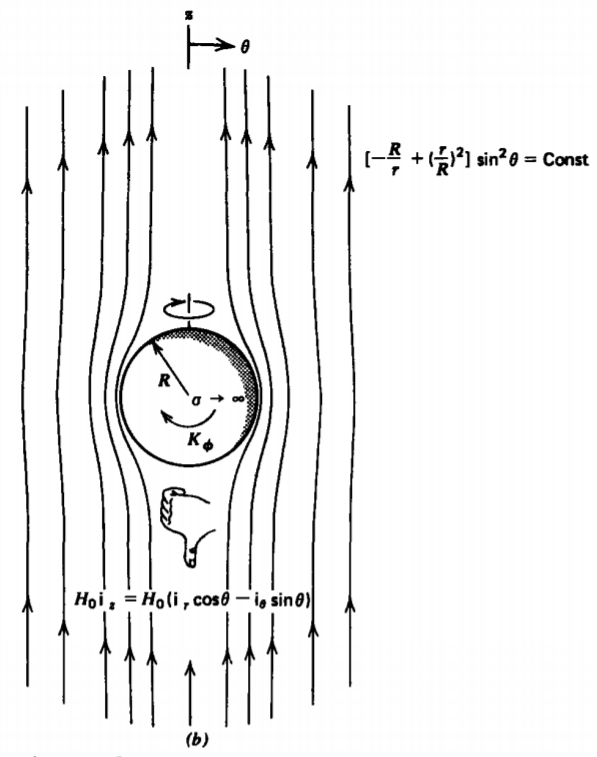
.(ii) If the sphere is perfectly conducting, the internal magnetic field is zero so that A = 0. The normal component of B right outside the sphere is then also zero:

\[H_{r}(r = R_{+}) = 0 \Rightarrow C = H_{0}R^{3}/2 \]

yielding the solution

\[\textbf{H} = H_{0} \bigg[ \(1 - \frac{R^{3}{r^{3}} \bigg) \cos \theta \textbf{i}_{r} - \bigg( 1 + \frac{R^{3}}{2r^{3}} \bigg) \sin \theta \textbf{i}_{\theta} \bigg], \: \: \: \: r > R \]

The interfacial surface current at r = R is obtained from the discontinuity in the tangential component of H:

\[K_{\phi} = H_{\phi} (r = R) = - \frac{3}{2}H_{0} \sin \theta \]

The current flows in the negative \(\phi\) direction around the sphere. The right-hand rule, illustrated in Figure 5-25b, shows that the resulting field from the induced current acts in the direction opposite to the imposed field. This opposition results in the zero magnetic field inside the sphere.

The field lines plotted in Figure 5-25b are purely tangential to the perfectly conducting sphere as required by (14)

(iii) If both regions are uniformly magnetized, the boundary conditions are

\[H_{\theta} (r = R_{+}) = H_{\theta} (r = R_{-}) \Rightarrow A = D + C/R^{3} \\ B_{r} (R = R_{+}) = B_{r}(r = R_{-}) \Rightarrow H_{r}(r = R_{+}) + M_{1} \cos \theta \\ H_{r} ( r = R_{-}) + M_{2} \cos \theta \]

with solutions

\[A = H_{0} + \frac{1}{3}(M_{1} - M_{2}) \\ C = \frac{R^{3}}{3} (M_{1} - M_{2}) \]

so that the magnetic field is

\begin{array}{l}
{\left[H_0+\frac{1}{3}\left(M_1-M_2\right)\right]\left[\cos \theta \mathbf{i}_r-\sin \theta \mathbf{i}_\theta\right]} \\
\quad=\left[H_0+\frac{1}{3}\left(M_1-M_2\right)\right] \mathbf{i}_z \quad r<R \\
\left(H_0-\frac{2 R^3}{3 r^3}\left(M_1-M_2\right)\right) \cos \theta \mathbf{i}_r \\
\quad-\left(H_0+\frac{R^3}{3 r^3}\left(M_1-M_2\right)\right) \sin \theta \mathbf{i}_\theta, \quad r>R
\end{array}

Because the magnetization is uniform in each region, the curl of M is zero everywhere but at the surface of the sphere, so that the volume magnetization current is zero with a surface magnetization current at r = R given by

\[\textbf{K}_{m} = \textbf{n} \times (\textbf{M}_{1} - \textbf{M}_{2}) \\ = \textbf{i}_{r} \times (M_{1} - M_{2}) \textbf{i}_{z} \\ = \textbf{i}_{r} \times (M_{1} - M_{2}) (\textbf{i}_{r} \cos \theta - \sin \theta \textbf{i}_{\theta}) = - (M_{1} - M_{2} ) \sin \theta \textbf{i}_{\phi} \]