5.8: Magnetic Fields and Forces

5-8-1 Magnetizable Media

A magnetizable medium carrying a free current \(\textbf{J}_{f}\) is placed within a magnetic field \(\textbf{B}\), which is a function of position. In addition to the Lorentz force, the medium feels the forces on all its magnetic dipoles. Focus attention on the rectangular magnetic dipole shown in Figure 5-26. The force on each current carrying leg is

\[\textbf{f} = \textbf{i} dl \times (B_{x} \textbf{i}_{x} + B_{y} \textbf{i}_{y} + B_{z} \textbf{i}_{z}) \\ \Rightarrow \textbf{f}(x) = - i \Delta y [ -B_{x} \textbf{i}_{z} + B_{z} \textbf{i}_{x}] \big|_{x} \\ \textbf{f}(x + \Delta x) = i \Delta y [ - B_{x} \textbf{i}_{z} + B_{z} \textbf{i}_{x}] \big|_{x + \Delta x} \\ \textbf{f} (y) = i \Delta x [B_{y} \textbf{i}_{z} - D_{z} \textbf{i}_{y}] \big|_{y} \\ \textbf{f} (y + \Delta y) = -i \Delta x [ B_{y} \textbf{i}_{z} - B_{z} \textbf{i}_{y}] \big|_{y + \Delta y} \]

so that the total force on the dipole is

\[\textbf{f} = \textbf{f} (x) + \textbf{f} (x + \Delta x) + \textbf{f} (y) + \textbf{f} ( y + \Delta y) \\ = - \Delta x \Delta y \bigg[ \frac{B_{z} (x + \Delta x) - B_{z} (x)}{\Delta x} \textbf{i}_{z} - \frac{B_{x} (x + \Delta x) - B_{x} (x)}{\Delta x} \textbf{i}_{z} + \frac{B_{z}(y + \Delta y) - B_{z} (y)}{\Delta y} \textbf{i}_{y} - \frac{B_{y}(y + \Delta y) - B_{y} (y)}{\Delta y} \textbf{i}_{z} \bigg] \]

Figure 5-26 A magnetic dipole in a magnetic field B.

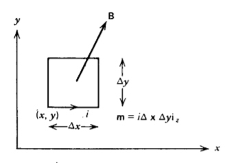
In the limit of infinitesimal \(\Delta x\) and \(\Delta y \) the bracketed terms define partial derivatives while the coefficient is just the magnetic dipole moment \(\textbf{m} = i \Delta x \Delta y \textbf{i}_{z}\) :

\[\lim_{\Delta x \rightarrow 0 \\ \Delta y \rightarrow 0} \textbf{f} = m_{z} \bigg[ \frac{\partial B_{z}}{\partial x} \textbf{i}_{x} - \bigg( \frac{\partial B_{x}}{\partial x} + \frac{\partial B_{y}}{\partial y} bigg) \textbf{i}_{z} + \frac{\partial B_{z}}{\partial y} \textbf{i}_{y} \bigg] \]

Ampere's and Gauss's law for the magnetic field relate the field components as

\[\nabla \cdot \textbf{B} = 0 \Rightarrow \frac{\partial B_{z}}{\partial z} = - \bigg( \frac{\partial B_{z}}{\partial x} + \frac{\partial B_{y}}{\partial y} \bigg) \]

\[\nabla \times \textbf{B} = \mu_{0}(\textbf{J}_{f} + \nabla \times \textbf{M}) = \mu_{0} \textbf{J}_{T} \Rightarrow \frac{\partial B_{z}}{\partial y} - \frac{\partial B_{y}}{\partial z} = \mu_{0} J_{Tx} \\ \frac{\partial B_{x}}{\partial z} - \frac{\partial B_{z}}{\partial x} = \mu_{0} J_{Ty} \\ \frac{\partial B_{y}}{\partial x} - \frac{\partial B_{x}}{\partial y} = \mu_{0}J_{Tz} \]

which puts (3) in the form

\[\textbf{f} = m_{z} \bigg( \frac{\partial B_{x}}{\partial z} \textbf{i}_{x} + \frac{\partial B_{y}}{\partial z} \textbf{i}_{y} + \frac{\partial B_{z}}{\partial z} \textbf{i}_{z} - \mu_{0}(J_{Ty} \textbf{i}_{x} - J_{Tx} \textbf{i}_{y}) \bigg) \\ = (\textbf{m} \cdot \nabla) \textbf{B} + \mu_{0} \textbf{m} \times \textbf{J}_{T} \]

where \(\textbf{J}_{T}\) is the sum of free and magnetization currents.

If there are N such dipoles per unit volume, the force density on the dipoles and on the free current is

\[\textbf{F} = N \textbf{f} = ( \textbf{M} \cdot \nabla) \textbf{B} + \mu_{0} \textbf{M} \times \textbf{J}_{T} + \textbf{J}_{f} \times \textbf{B} \\ = \mu_{0} (\textbf{M} \cdot \nabla) ( \textbf{H} + \textbf{M}) + \mu_{0} \textbf{M} \times (\textbf{J}_{f} + \nabla \times \textbf{M}) + \mu_{0} \textbf{J}_{f} \times (\textbf{H} + \textbf{M}) \\ = \mu_{0} (\textbf{M} \cdot \nabla) (\textbf{H} + \textbf{M}) + \mu_{0} \textbf{M} \times (\nabla \times \textbf{M}) + \mu_{0} \textbf{J}_{f} \times \textbf{H} \]

Using the vector identity

\[\textbf{M} \times (\nabla \times \textbf{M}) = - (\textbf{M} \cdot \nabla) \textbf{M} + \frac{1}{2} \nabla (\textbf{M} \cdot \textbf{M}) \]

(7) can be reduced to

\[\textbf{F} = \mu_{0} (\textbf{M} \cdot \nabla) \textbf{H} + \mu_{0} \textbf{J}_{f} \times \textbf{H} + \nabla \bigg( \frac{\mu_{0}}{2} \textbf{m} \cdot \textbf{M} \bigg) \]

The total force on the body is just the volume integral of F:

\[\textbf{f} = \int_{\textrm{V}} \textbf{F} d \textrm{V} \]

In particular, the last contribution in (9) can be converted to a surface integral using the gradient theorem, a corollary to the divergence theorem (see Problem 1-15a):

\[\int_{\textrm{V}} \nabla \bigg( \frac{\mu_{0}}{2} \textbf{M} \cdot \textbf{M} \bigg) d \textrm{V} = \oint_{S} \frac{\mu_{0}}{2} \textbf{M} \cdot \textbf{M} d \textrm{S} \]

Since this surface S surrounds the magnetizable medium, it is in a region where M = 0 so that the integrals in (11) are zero. For this reason the force density of (9) is written as

\[\textbf{F} = \mu_{0} ( \textbf{M} \cdot \nabla) \textbf{H} + \mu_{0} \textbf{J}_{f} \times \textbf{H} \]

It is the first term on the right-hand side in (12) that accounts for an iron object to be drawn towards a magnet. Magnetizable materials are attracted towards regions of higher H.

5-8-2 Force on a Current Loop

(a) Lorentz Force Only

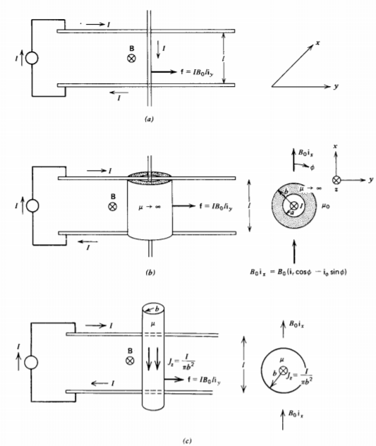
Two parallel wires are connected together by a wire that is free to move, as shown in Figure 5-27a. A current I is imposed and the whole loop is placed in a uniform magnetic field \(B_{0} \textbf{i}_{x}\). The Lorentz force on the moveable wire is

\[f_{y} = I B_{0} l \]

where we neglect the magnetic field generated by the current, assuming it to be much smaller than the imposed field \(B_{0}\).

(b) Magnetization Force Only

The sliding wire is now surrounded by an infinitely permeable hollow cylinder of inner radius a and outer radius b, both being small compared to the wire's length l, as in Figure 5-27b. For distances near the cylinder, the solution is approximately the same as if the wire were infinitely long. For r>0 there is no current, thus the magnetic field is curl and divergence free within each medium so that the magnetic scalar potential obeys Laplace's equation as in Section 5-7-2. In cylindrical geometry we use the results of Section 4-3 and try a scalar potential of the form

\[\chi = \bigg( A \textrm{r} + \frac{C}{\textrm{r}} \bigg) \cos \phi \]

Figure 5-27 (a) The Lorentz-force on a current carrying wire in a magnetic field. (b) If the current-carrying wire is surrounded by an infinitely permeable hollow cylinder, there is no Lorentz force as the imposed magnetic field is zero where the current is. However, the magnetization force on the cylinder is the same as in (a). (c) The total force on a current-carrying magnetically permeable wire is also unchanged.

in each region, where \(\textbf{B} = \nabla_{\chi}\) because \(\nabla \times \textbf{B} = 0\). The constants are evaluated by requiring that the magnetic field approach the imposed field \(B_{0} \textbf{i}_{x}\) at r = \(\infty\) and be normally incident onto the infinitely permeable cylinder at r = a and r = b. In addition, we must add the magnetic field generated by the line current. The magnetic field in each region is then

(See Problem 32a):

\[\textbf{B} = \left \{ \begin{matrix} \frac{\mu_{0}I}{2 \pi \textrm{r}} \textbf{i}_{\phi}, & 0 < \textrm{r} < a \\ \frac{2B_{0}b^{2}}{b^{2}-a^{2}} \bigg[ \bigg( 1 - \frac{a^{2}}{\textrm{r}^{2}} \bigg) \cos \phi \textbf{i}_{\textrm{r}} - \bigg( 1 + \frac{a^{2}}{\textrm{r}^{2}} \bigg) \sin \phi \textbf{i}_{\phi} \bigg] + \frac{\mu I}{2 \pi \textrm{r}} \textbf{i}_{\phi}, & a < \textrm{r} < b \\ B_{0} \bigg[ \bigg( 1 + \frac{b^{2}}{\textrm{r}^{2}} \bigg) \cos \phi \textbf{i}_{\textrm{r}} - \bigg( 1 - \frac{b^{2}}{\textrm{r}^{2}} \bigg) \sin \phi \textbf{i}_{\phi} \bigg] + \frac{\mu_{0} I}{2 \pi \textrm{r}} \textbf{i}_{\phi}, & \textrm{r} > b \end{matrix} \right. \]

Note the infinite flux density in the iron ( \(\mu \rightarrow \infty\) ) due to the line current that sets up the finite H field. However, we see that none of the imposed magnetic field is incident upon the current carrying wire because it is shielded by the infinitely permeable cylindrical shell so that the Lorentz force contribution on the wire is zero. There is, however, a magnetization force on the cylindrical shell where the internal magnetic field H is entirely due to the line current, \(H_{\phi} = I/2 \pi\)r because with \(\mu \rightarrow \infty\), the contribution due to \(B_{0}\) is negligibly small:

\[\textbf{F} = \mu_{0} (\textbf{M} \cdot \nabla) \textbf{H} \\ = \mu_{0} \bigg( M_{\textrm{r}} \frac{\partial}{\partial \textrm{r}} (H_{\phi} \textbf{i}_{\phi}) + \frac{M_{\phi}}{\textrm{r}} \frac{\partial}{\partial \phi} (H_{\phi} \textbf{i}_{\phi}) \bigg) \]

Within the infinitely permeable shell the magnetization and H fields are

\[H_{\phi} = \frac{I}{2 \pi r} \\ \mu_{0} M_{\textrm{r}} = B_{\textrm{r}} - \mu_{0} H \nearrow^{0}_{\textrm{r}} = \frac{2 B_{0}b^{2}}{b^{2} - a^{2}} \bigg( 1 - \frac{a^{2}}{\textrm{r}^{2}} \bigg) \cos \phi \\ \mu_{0} M_{\phi} = B_{\phi} - \mu_{0} H_{\phi} = - \frac{2 B_{0}b^{2}}{(b^{2}-a^{2})} \bigg( 1 + \frac{a^{2}}{\textrm{r}^{2}} \bigg) \sin \phi + \frac{(\mu - \mu_{0})I}{2 \pi \textrm{r}} \]

Although \(H_{\phi}\) only depends on r, the unit vector \(\textbf{i}_{phi}\) depends on \(\phi\).

\[\textbf{i}_{\phi} = (-\sin \phi \textbf{i}_{x} + \cos \phi \textbf{i}_{y}) \]

so that the force density of (16) becomes

\[\textbf{F} = - \frac{B_{\textrm{r}}I}{2 \pi \textrm{r}^{2}} \textbf{i}_{\phi} + \frac{(B_{\phi} - \mu_{0} H_{\phi})I}{2 \pi \textrm{r}^{2}} \frac{d}{d \phi} (\textbf{i}_{\phi}) \\ \frac{I}{2 \pi textrm{r}^{2}} [ - B_{\textrm{r}} (- \sin \phi \textbf{i}_{x} + \cos \phi \textbf{i}_{y}) \\ + (B_{\phi} - \mu_{0} H_{\phi})(- \cos \phi \textbf{i}_{x} - \sin \phi \textbf{i}_{y})] \\ = \frac{I}{2 \pi \textrm{r}^{2}} \bigg( - \frac{2 B_{0} b^{2}}{b^{2}-a^{2}} \bigg[ \bigg( 1 - \frac{a^{2}}{\textrm{r}^{2}} \bigg) \cos \phi (- \sin \phi \textbf{i}_{x} + \cos \phi \textbf{i}_{y}) \\ - \bigg( 1 + \frac{a^{2}}{\textrm{r}^{2}} \bigg) \sin \phi (\cos \phi \textbf{i}_{x} + \sin \phi \textbf{i}_{y}) \bigg] \\ + \frac{(\mu - \mu_{0}) I}{2 \pi \textrm{r}} (\cos \phi \textbf{i}_{x} + \sin \phi \textbf{i}_{y}) \bigg) \\ = \frac{I}{2 \pi \textrm{r}^{2}} \bigg[ - \frac{2 B_{0} b^{2}}{b^{2} - a^{2}} \bigg( -2 \sin \phi \cos \phi \textbf{i}_{x} - \frac{2a^{2}}{\textrm{r}^{2}} \textbf{i}_{y} \bigg) + \frac{(\mu - \mu_{0})I}{2 \pi \textrm{r}} (\cos \phi \textbf{i}_{x} + \sin \phi \textbf{i}_{y}) \bigg) \]

The total force on the cylinder is obtained by integrating (19) over r and \(\phi\).

\[\textbf{f} = \int_{\phi = 0}^{2\pi} \int_{\textrm{r} = a}^{b} \textbf{F} l \: \textrm{r} \: d \textrm{r} \: d \phi \]

All the trigonometric terms in (19) integrate to zero over \(\phi\) so that the total force is

\[f_{y} = \frac{2 B_{0} b^{2} I l}{(b^{2} - a^{2}) \int_{\textrm{r} = a}}^{b} \frac{a^{2}}{\textrm{r}^{3}} d \textrm{r} \\ = - \frac{B_{0}b^{2} I l}{(b^{2} - a^{2})} \frac{a^{2}}{\textrm{r}^{2}} \bigg|_{a}^{b} \\ = I B_{0} l \]

The force on the cylinder is the same as that of an unshielded current-carrying wire given by (13). If the iron core has a finite permeability, the total force on the wire (Lorentz force) and on the cylinder (magnetization force) is again equal to (13). This fact is used in rotating machinery where currentcarrying wires are placed in slots surrounded by highly permeable iron material. Most of the force on the whole assembly is on the iron and not on the wire so that very little restraining force is necessary to hold the wire in place. The force on a current-carrying wire surrounded by iron is often calculated using only the Lorentz force, neglecting the presence of the iron. The correct answer is obtained but for the wrong reasons. Actually there is very little B field near the wire as it is almost surrounded by the high permeability iron so that the Lorentz force on the wire is very small. The force is actually on the iron core.

(c) Lorentz and Magnetization Forces

If the wire itself is highly permeable with a uniformly distributed current, as in Figure 5-27c, the magnetic field is (see Problem 32a)

\[\textbf{H} = \left \{ \begin{matrix} \frac{2 B_{0}}{\mu + \mu_{0}} (\textbf{i}_{\textrm{r}} \cos \phi - \textbf{i}_{\phi} \sin \theta) + \frac{I \textrm{r}}{2 \pi b^{2}} \textbf{i}_{\phi} & \: \\ = \frac{2B_{0}}{\mu + \mu_{0}} \textbf{i}_{x} + \frac{I}{2 \pi b^{2}} (-y \textbf{i}_{x} + x \textbf{i}_{y}), & \textrm{r} < b \\ \frac{B_{0}}{\mu_{0}} \bigg[ \bigg( 1 + \frac{b^{2}}{\textrm{r}^{2}} \frac{\mu - \mu_{0}}{\mu + \mu_{0}} \bigg) \cos \phi \textbf{i}_{\textrm{r}} & \: \\ - \bigg( 1 - \frac{b^{2}}{\textrm{r}^{2}} \frac{\mu - \mu_{0}}{\mu + \mu_{0}} \bigg) \sin \phi \textbf{i}_{\phi} \bigg] + \frac{I}{2 \pi \textrm{r}} \textbf{i}_{\phi}, & \textrm{r} > b \end{matrix} \right. \]

It is convenient to write the fields within the cylinder in Cartesian coordinates using (18) as then the force density given by (12) is

\[\textbf{F} = \mu_{0}(\textbf{M} \cdot \nabla) \textbf{H} + \mu_{0} \textbf{J}_{f} \times \textbf{H} \\ = (\mu - \mu_{0}) (\textbf{H} \cdot \nabla) \textbf{H} + \frac{\mu_{0} I}{\pi b^{2}} \textbf{i}_{z} \times \textbf{H} \\ = (\mu - \mu_{0}) (\textbf{H} \cdot \nabla) \textbf{H} + \frac{\mu_{0} I}{\pi b^{2}} \textbf{i}_{z} \times \textbf{H} \\ = (\mu - \mu_{0}) \bigg( H_{x} \frac{\partial}{\partial x} + H_{y} \frac{\partial}{\partial y} \bigg) (H_{x} \textbf{i}_{x} + H_{y} \textbf{i}_{y}) + \frac{\mu_{0}I}{\pi b^{2}} (H_{x} \textbf{i}_{y} - H_{y} \textbf{i}_{x}) \]

Since within the cylinder (r < b) the partial derivatives of H are

\[\frac{\partial H_{x}}{\partial x} = \frac{\partial H_{y}}{\partial y} = 0 \\ \frac{\partial H_{x}}{\partial y} = - \frac{\partial H_{y}}{\partial x} = - \frac{I}{2 \pi b^{2}} \]

(23) reduces to

\[\textbf{F} = (\mu - \mu_{0}) \bigg( H_{x} \frac{\partial H_{y}}{\partial x} \textbf{i}_{y} + H_{y} \frac{\partial H_{x}}{\partial y} \textbf{i}_{x} \bigg) + \frac{\mu_{0}I}{\pi b^{2}} (H_{x} \textbf{i}_{y} - H_{y} \textbf{i}_{x}) \\ = \frac{I}{2 \pi b^{2}} (\mu + \mu_{0}) (H_{x} \textbf{i}_{y} - H_{y} \textbf{i}_{x}) \\ = \frac{I (\mu + \mu_{0})}{2 \pi b^{2}} \bigg[ \bigg( \frac{2 B_{0}}{\mu + \mu_{0}} - \frac{Iy}{2 \pi b^{2}} \bigg) \textbf{i}_{y} - \frac{Ix}{2 \pi b^{2}} \textbf{i}_{x} \bigg] \]

Realizing from Table 1-2 that

\[y \textbf{i}_{y} + x \textbf{i}_{x} = \textrm{r} [ \sin \phi \textbf{i}_{y} + \cos \phi \textbf{i}_{x}] = \textrm{r} \textbf{i}_{\textrm{r}} \]

the force density can be written as

\[\textbf{F} = \frac{IB_{0}}{\pi b^{2}} \textbf{i}_{y} - \frac{I^{2} (\mu + \mu_{0})}{(2 \pi b^{2})^{2}} \textrm{r} (\sin \phi \textbf{i}_{y} + \cos \phi \textbf{i}_{x}) \]

The total force on the permeable wire is

\[\textbf{f} = \int_{\phi = 0}^{2 \pi} \int_{\textrm{r} = 0}^{b} \textbf{F} l r d \textrm{r} \: d \phi \]

We see that the trigonometric terms in (27) integrate to zero so that only the first term contributes:

\[f_{y} = \frac{I B_{0} l}{\pi b^{2}} \int_{\phi = 0}^{2 \pi} \int_{\textrm{r = 0}}^{b} \textrm{r} \: d \textrm{r} \: d \phi \\ = I B_{0} l \]

The total force on the wire is independent of its magnetic permeability.