7.2: Conservation of Energy

Poynting's Theorem

We expand the vector quantity

\begin{align} \nabla\cdot \left ( \textbf{E}\times \textbf{H} \right ) & =\textbf{H}\cdot \left (\nabla\times \textbf{E} \right )-\textbf{E}\cdot \left ( \nabla\times\textbf{H} \right )\\ & =-\textbf{H}\cdot \frac{\partial \textbf{B}}{\partial t}-\textbf{E}\cdot \frac{\partial \textbf{D}}{\partial t}-\textbf{E}\cdot \textbf{J}_{f} \nonumber \end{align}

where we change the curl terms using Faraday's and Ampere's laws.

For linear homogeneous media, including free space, the constitutive laws are

\[ \textbf{D}=\varepsilon \textbf{E}, \quad \textbf{B}=\mu \textbf{H} \]

so that (1) can be rewritten as

\[ \nabla\cdot \left ( \textbf{E}\times \textbf{H} \right )+\frac{\partial }{\partial t}\left ( \frac{1}{2}\varepsilon \textbf{E}^{2}+\frac{1}{2}\mu \textbf{H}^{2} \right )=\textbf{E}\cdot \textbf{J}_{f} \]

which is known as Poynting's theorem. We integrate (3) over a closed volume, using the divergence theorem to convert the first term to a surface integral:

\[ \underbrace{\oint_{\textbf{S}}\left ( \textbf{E}\times \textbf{H} \right )\cdot \textbf{dS}}_{\int_{\textbf{V}}\nabla\cdot \left ( \textbf{E}\times \textbf{H} \right )\textbf{dV}}+\frac{d}{dt}\int_{\textbf{V}}\left (  \frac{1}{2}\varepsilon \textbf{E}^{2}+\frac{1}{2}\mu \textbf{H}^{2} \right )\textbf{dV}=-\int_{\textbf{V}}^{}\textbf{E}\cdot \textbf{J}_{f}\textbf{dV} \]

We recognize the time derivative in (4) as operating on the electric and magnetic energy densities, which suggests the interpretation of (4) as

\[ P_{out}+\frac{dW}{dt}=-P_{d} \]

where \(P_{out}\), is the total electromagnetic power flowing out of the volume with density

\[ S=\textbf{E}\times \textbf{H}\,\,\mathrm{watts/m^{2}[kg\cdot s^{-3}]} \]

where \(S\) is called the Poynting vector, \(W\) is the electromagnetic stored energy, and \(P_d\) is the power dissipated or generated:

\[ P_{out} =\oint_{\textbf{S}}\left ( \textbf{E}\times \textbf{H} \right )\cdot \textbf{dS}=\oint_{\textbf{S}}S\cdot \textbf{dS} \\W=\int_{\textbf{V}}[\frac{1}{2}\varepsilon \textbf{E}^{2}+\frac{1}{2}\mu \textbf{H}^{2}]d\textbf{V}\\P_d=\oint_{\textbf{V}}\textbf{E}\cdot \textbf{J}_{f}d\textbf{V} \]

If \(\textbf{E}\) and \(\textbf{J}_{f}\) are in the same direction as in an Ohmic conductor \(\left ( \textbf{E}\cdot \textbf{J}_{f}=\sigma E^{2} \right )\), then \(P_d\) is positive, representing power dissipation since the right-hand side of (5) is negative. A source that supplies power to the volume has \(\textbf{E}\) and \(\textbf{J}_{f}\) in opposite directions so that \(P_d\) is negative.

A Lossy Capacitor

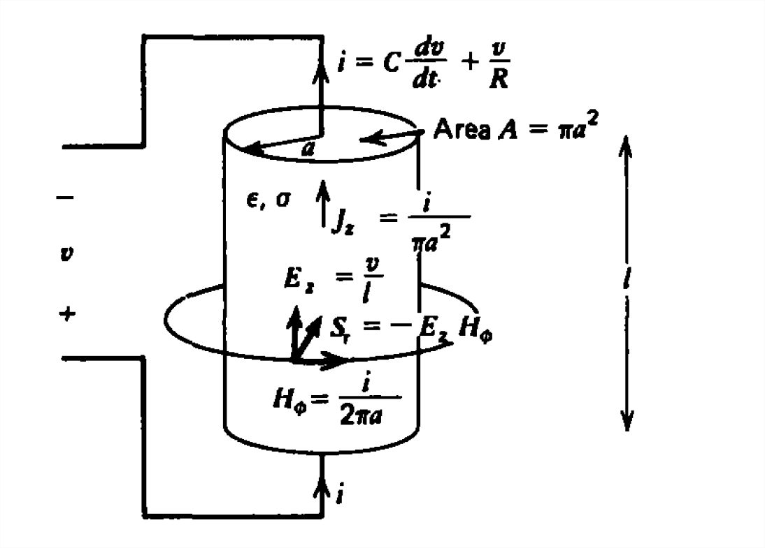
Poynting's theorem offers a different and to some a paradoxical explanation of power flow to circuit elements. Consider the cylindrical lossy capacitor excited by a time varying voltage source in Figure 7-1. The terminal current has both Ohmic and displacement current contributions:

\[ i=\frac{\varepsilon A}{l}\frac{dv}{dt}+\frac{\sigma Av}{l}=C\frac{dv}{dt}+\frac{v}{R},\quad C=\frac{\varepsilon A}{l},\quad R=\frac{l}{\sigma A} \]

From a circuit theory point of view we would say that the power flows from the terminal wires, being dissipated in the

Figure 7-1 The power delivered to a lossy cylindrical capacitor \(vi\) is partly dissipated by the Ohmic conduction and partly stored in the electric field. This power can also be thought to flow-in radially from the surrounding electric and magnetic fields via the Poynting vector \(\textbf{S}=\textbf{E}\times \textbf{H}\).

resistance and stored as electrical energy in the capacitor:

\[ P=vi=\frac{v^{2}}{R}+\frac{d}{dt}(\frac{1}{2}Cv^{2}) \]

We obtain the same results from a field's viewpoint using Poynting's theorem. Neglecting fringing, the electric field is simply

\[ E_z=v/l \]

while the magnetic field at the outside surface of the resistor is generated by the conduction and displacement currents:

\[ \oint_{L}\textbf{H}\cdot \textbf{dl} = \int_{\textbf{S}}\left ( J_z +\varepsilon \frac{\partial E_z}{\partial t}\right )d\textbf{S}\Rightarrow H_{\phi }2\pi a=\frac{\sigma Av}{l}+\frac{\varepsilon}{l}A\frac{dv}{dt}=i \]

where we recognize the right-hand side as the terminal current in (8),

\[ H_{\phi }=i/\left ( 2\pi a \right ) \]

The power flow through the surface at \( r = a\) surrounding the resistor is then radially inward,

\[ \oint_{\textbf{S}}\left ( \textbf{E}\times \textbf{H} \right )\cdot \textbf{dS}= -\int_{\textbf{S}}\frac{v}{l}\frac{i}{2\pi a}a\,d\phi dz= -vi \]

and equals the familiar circuit power formula. The minus sign arises because the left-hand side of (13) is the power out of the volume as the surface area element \(\textbf{dS}\) points radially outwards. From the field point of view, power flows into the lossy capacitor from the electric and magnetic fields outside the resistor via the Poynting vector. Whether the power is thought to flow along the terminal wires or from the surrounding fields is a matter of convenience as the results are identical. The presence of the electric and magnetic fields are directly due to the voltage and current. It is impossible to have the fields without the related circuit variables.

Power in Electric Circuits

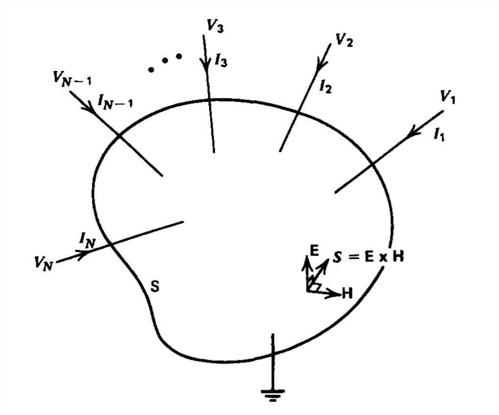
We saw in (13) that the flux of \(S\) entering the surface surrounding a circuit element just equals \(vi\). We can show this for the general network with \(N\) terminals in Figure 7-2 using the quasi-static field laws that describe networks outside the circuit elements:

\[ \nabla \times \textbf{E}=0\Rightarrow \textbf{E}=-\nabla V\\
\nabla \times \textbf{H}=\textbf{J}_f\Rightarrow \nabla\cdot \textbf{J}_f=0   \]

We then can rewrite the electromagnetic power into a surface as

\[ \begin{align} P_{in} & = -\oint_{\textbf{S}}\textbf{E}\times \textbf{H}\cdot \textbf{dS} \\ &  = -\int_{\textbf{V}}\nabla\cdot \left ( \textbf{E}\times \textbf{H} \right )d\textbf{V} \nonumber \\ &  =  \int_{\textbf{V}}\nabla\cdot \left ( \nabla V\times \textbf{H} \right )d\textbf{V}  \nonumber \nonumber \end{align} \]

Figure 7-2 The circuit power into an \(N\) terminal network \(\sum_{k=1}^{N} V_k I_k \) equals the electromagnetic power flow into the surface surrounding the network, \(-\oint_{\textbf{S}}\textbf{E}\times \textbf{H}\cdot \textbf{dS}\).

where the minus is introduced because we want the power in and we use the divergence theorem to convert the surface integral to a volume integral. We expand the divergence term as

\[ \begin{align} \nabla\cdot \left ( \nabla V\times \textbf{H} \right ) & =\textbf{H}\cdot \left (\overset{0}{\widehat{\nabla \times \nabla V}} \right )-\nabla V\cdot \left ( \nabla\times \textbf{H} \right ) \\ &=-\textbf{J}_f\cdot \nabla V=-\nabla\cdot \left ( \textbf{J}_f V \right ) \nonumber \end{align} \]

where we use (14).

Substituting (16) into (15) yields

\[ \begin{align} P_{in} & = -\int_{\textbf{V}}\nabla \cdot \left ( \textbf{J}_f V \right )dV \\ &=\oint_{\textbf{S}} \textbf{J}_f V \cdot \textbf{dS} \nonumber \end{align}
\]

where we again use the divergence theorem. On the surface \(S\), the potential just equals the voltages on each terminal wire allowing \(V\) to be brought outside the surface integral:

\[ \begin{align} P_{in} & = \sum_{k=1}^{N}-V_k\oint_{\textbf{S}}\textbf{J}_f\cdot \textbf{dS} \\ &= \sum_{k=1}^{N} V_k I_k  \nonumber \end{align} \]

where we recognize the remaining surface integral as just being the negative (remember \(\textbf{dS}\) points outward) of each terminal current flowing into the volume. This formula is usually given as a postulate along with Kirchoff's laws in most circuit theory courses. Their correctness follows from the quasi-static field laws that are only an approximation to more general phenomena which we continue to explore.

The Complex Poynting's Theorem

For many situations the electric and magnetic fields vary sinusoidally with time:

\[ \textbf{E}\left ( \textbf{r},t \right )=\textbf{Re}\left [ \mathbf{\hat{E}}\left ( \textbf{r} \right )e^{j\omega t} \right ]\\ \textbf{H}\left ( \textbf{r},t \right )=\textbf{Re}\left [ \mathbf{\hat{H}}\left ( \textbf{r} \right )e^{j\omega t} \right ] \]

where the caret is used to indicate a complex amplitude that can vary with position \(\textbf{r}\). The instantaneous power density is obtained by taking the cross product of \(\textbf{E}\) and \(\textbf{H}\). However, it is often useful to calculate the time-average power density \(< \textbf{S} >\), where we can avoid the lengthy algebraic and trigonometric manipulations in expanding the real parts in (19).

A simple rule for the time average of products is obtained by realizing that the real part of a complex number is equal to one half the sum of the complex number and its conjugate (denoted by a superscript asterisk). The power density is then

\[ \begin{align}\textbf{S}\left ( \textbf{r}, t \right )& =\textbf{E}\left ( \textbf{r}, t \right )\times \textbf{H}\left ( \textbf{r}, t \right ) \\ &=\frac{1}{4}\left [ \mathbf{\hat{E}}\left ( \textbf{r} \right )e^{j\omega t}+ \mathbf{\hat{E}}^{*}\left ( \textbf{r} \right )e^{-j\omega t}\right ]\times \left [ \mathbf{\hat{H}}\left ( \textbf{r} \right )e^{j\omega t}+ \mathbf{\hat{H}}^{*}\left ( \textbf{r} \right )e^{-j\omega t}\right ] \nonumber \\ &=\frac{1}{4}\left [ \mathbf{\hat{E}}\left ( \textbf{r} \right )\times  \mathbf{\hat{H}}\left ( \textbf{r} \right )e^{2j\omega t}+ \mathbf{\hat{E}}^{*}\left ( \textbf{r} \right ) \times \mathbf{\hat{H}}\left ( \textbf{r} \right )+  \mathbf{\hat{E}}\left ( \textbf{r} \right ) \times \mathbf{\hat{H}}^{*}\left ( \textbf{r} \right ) +\mathbf{\hat{E}}^{*}\left ( \textbf{r} \right ) \times \mathbf{\hat{H}}^{*}\left ( \textbf{r} \right )e^{-2j\omega t}\right ]  \nonumber \end{align} \]

The time average of (20) is then

\[ \begin{align}< \textbf{S} > & =\frac{1}{4}\left [\mathbf{\hat{E}}^{*}\left ( \textbf{r} \right ) \times \mathbf{\hat{H}}\left ( \textbf{r} \right ) +\mathbf{\hat{E}}\left ( \textbf{r} \right ) \times \mathbf{\hat{H}}^{*}\left ( \textbf{r} \right )\right ]  \\ & = \frac{1}{2}\textbf{Re}\left [ \mathbf{\hat{E}}\left ( \textbf{r} \right ) \times \mathbf{\hat{H}}^{*}\left ( \textbf{r} \right ) \right ] \nonumber \\ & = \frac{1}{2}\textbf{Re}\left [ \mathbf{\hat{E}}^{*}\left ( \textbf{r} \right ) \times \mathbf{\hat{H}}\left ( \textbf{r} \right ) \right ] \nonumber \end{align} \]

as the complex exponential terms \(e^{\pm 2j\omega t}\) average to zero over a period \(T = 2\pi /\omega\) and we again realized that the first bracketed term on the right-hand side of (21) was the sum of a complex function and its conjugate.

Motivated by (21) we define the complex Poynting vector as

\[ \mathbf{\hat{S}}=\frac{1}{2}\mathbf{\hat{E}}\left ( \textbf{r} \right ) \times \mathbf{\hat{H}}^{*}\left ( \textbf{r} \right ) \]

whose real part is just the time-average power density.

We can now derive a complex form of Poynting's theorem by rewriting Maxwell's equations for sinusoidal time variations as

\[ \begin{align}
\nabla\times \mathbf{\hat{E}}\left ( \textbf{r} \right )&=-j\omega \mu \mathbf{\hat{H}}\left ( \textbf{r} \right ) \\
\nabla\times \mathbf{\hat{H}}\left ( \textbf{r} \right )& =\mathbf{\hat{J}}_{f}\left ( \textbf{r} \right )+j\omega\varepsilon \mathbf{\hat{E}}\left ( \textbf{r} \right ) \nonumber \\
\nabla\times \mathbf{\hat{E}}\left ( \textbf{r} \right )&=\hat{\rho }_{f}\left ( \textbf{r} \right )/\varepsilon \nonumber \\
\nabla\times \mathbf{\hat{B}}\left ( \textbf{r} \right )&=0 \nonumber \end{align} \]

and expanding the product

\[ \begin{align} \nabla\times \mathbf{\hat{S}} &=\nabla\cdot \left [  \frac{1}{2}\mathbf{\hat{E}}\left ( \textbf{r} \right ) \times \mathbf{\hat{H}}^{*}\left ( \textbf{r} \right )\right ]   \\ &=\frac{1}{2}\left [ \mathbf{\hat{H}}^{*}\left ( \textbf{r} \right )\cdot \nabla\times \mathbf{\hat{E}}\left ( \textbf{r} \right ) - \mathbf{\hat{E}}\left ( \textbf{r} \right )\cdot \nabla\times \mathbf{\hat{H}}^{*}\left ( \textbf{r} \right )\right ] \nonumber \\ &=\frac{1}{2}\left [ -j\omega \mu \left | \mathbf{\hat{H}}\left ( \textbf{r} \right ) \right |^{2} +j\omega \varepsilon \left | \mathbf{\hat{E}}\left ( \textbf{r} \right ) \right |^{2}-\frac{1}{2}\mathbf{\hat{E}}\left ( \textbf{r} \right )\cdot \mathbf{\hat{J}}_{f}^{*}\left ( \textbf{r} \right )\right ] \nonumber \end{align} \]

which can be rewritten as

\[\nabla\times \mathbf{\hat{S}} +2j\omega \left [ < \omega _{m}> -< \omega_{e} >  \right ]=-\hat{P}_{d} \]

where

\[ \begin{align}
< \omega _{m}> &=\frac{1}{4}\mu \left | \mathbf{\hat{H}}\left ( \textbf{r} \right ) \right |^{2} \\
< \omega_{e} > &=\frac{1}{4}\varepsilon \left | \mathbf{\hat{E}}\left ( \textbf{r} \right ) \right |^{2} \nonumber \\
\hat{P}_{d} & =\frac{1}{2}\mathbf{\hat{E}}\left ( \textbf{r} \right )\cdot \mathbf{\hat{J}}_{f}^{*}\left ( \textbf{r} \right ) \nonumber \end{align} \]

We note that \(< \omega _{m}\) and \(< \omega_{e} >\) are the time-average magnetic and electric energy densities and that the complex Poynting's theorem depends on their difference rather than their sum.