7.3: Transverse Electromagnetic Waves

Plane Waves

Let us try to find solutions to Maxwell's equations that only depend on the \(z\) coordinate and time in linear media with permittivity \(\varepsilon\) and permeability \(\mu\). In regions where there are no sources so that \(\rho _{f}=0\), \(\textbf{J}_{f}=0\), Maxwell's equations then reduce to

\[-\frac{\partial E_{y}}{\partial z}\textbf{i}_{x}+\frac{\partial E_{x}}{\partial z}\textbf{i}_{y}=-\mu \frac{\partial \textbf{H}}{\partial t} \]

\[ -\frac{\partial H_{y}}{\partial z}\textbf{i}_{x}+\frac{\partial H_{x}}{\partial z}\textbf{i}_{y}=\varepsilon  \frac{\partial \textbf{E}}{\partial t} \]

\[ \varepsilon \frac{\partial E_{z}}{\partial z}=0 \]

\[\mu \frac{\partial H_{z}}{\partial z}=0 \]

These relations tell us that at best \(E_{z}\), and \(H_{z}\), are constant in time and space. Because they are uncoupled, in the absence of sources we take them to be zero. By separating vector components in (1) and (2) we see that \(E_{x}\) is coupled to \(H_{y}\), and \(E_{y}\), is coupled to \(H_{x}\):

\[ \frac{\partial E_{x}}{\partial z}=-\mu \frac{\partial H_{y}}{\partial t}, \quad \frac{\partial E_{y}}{\partial z}=\mu\frac{\partial H_{x}}{\partial t}\\ \frac{\partial H_{y}}{\partial z}=-\varepsilon \frac{\partial E_{x}}{\partial t}, \quad \frac{\partial H_{x}}{\partial z}=\varepsilon \frac{\partial E_{y}}{\partial t}  \]

forming two sets of independent equations. Each solution has perpendicular electric and magnetic fields. The power flow \(\textbf{S}=\textbf{E}\times \textbf{H}\) for each solution is \(z\) directed also being perpendicular to \(\textbf{E}\) and \(\textbf{H}\). Since the fields and power flow are mutually perpendicular, such solutions are called transverse electromagnetic waves (TEM). They are waves because if we take \(\partial/\partial z\) of the upper equations and \(\partial/\partial t\) of the lower equations and solve for the electric fields, we obtain one-dimensional wave equations:

\[ \frac{\partial^2 E_{x}}{\partial z^2}=\frac{1}{c^{2}}\frac{\partial^2 E_{x}}{\partial t^2},\quad \frac{\partial^2 E_{y}}{\partial z^2}=\frac{1}{c^{2}}\frac{\partial^2 E_{y}}{\partial t^2} \]

where \(c\) is the speed of the wave,

\[ c=\frac{1}{\sqrt{\varepsilon \mu }}=\frac{1}{\sqrt{\varepsilon _{0}\mu _{0}}\sqrt{\varepsilon _{r}\mu _{r}}}\approx \frac{3\times 10^{8}}{\sqrt{\varepsilon _{r}\mu _{r}}}\,\mathrm{m/sec} \]

In free space, where \(\varepsilon _{r}=1\) and \(\mu _{r}=1\), this quantity equals the speed of light in vacuum which demonstrated that light is a transverse electromagnetic wave. If we similarly take \(\partial/\partial t\) of the upper and \(\partial/\partial z\) of the lower equations in (5), we obtain wave equations in the magnetic fields:

\[ \frac{\partial^2 H_{y}}{\partial z^2}=\frac{1}{c^{2}}\frac{\partial^2 H_{y}}{\partial t^2},\quad \frac{\partial^2 H_{x}}{\partial z^2}=\frac{1}{c^{2}}\frac{\partial^2 H_{x}}{\partial t^2} \]

The Wave Equation

(a) Solutions

These equations arise in many physical systems, so their solutions are well known. Working with the \(\)E and \(\)H, equations, the solutions are

\[ E_{x}\left ( z,t \right )=E_{+}\left ( t-z/c \right )+E_{-}\left ( t+z/c  \right )\\
H_{y}\left ( z,t \right )=H_{+}\left ( t-z/c \right )+H_{-}\left ( t+z/c  \right ) \]

where the functions \(E_{+}\), \(E_{-}\), \(H_{+}\), and \(H_{-}\) depend on initial conditions in time and boundary conditions in space. These solutions can be easily verified by defining the arguments \(\alpha\) and \(\beta \) with their resulting partial derivatives as

\[ \alpha = t-\frac{z}{c}\Rightarrow \frac{\partial \alpha }{\partial t}=1,\quad \frac{\partial \alpha }{\partial z}=-\frac{1}{c}\\\beta =t+\frac{z}{c}\Rightarrow \frac{\partial \beta }{\partial t} =1,\quad \frac{\partial \beta }{\partial z}=\frac{1}{c} \]

and realizing that the first partial derivatives of \(E_{x}\left ( z,t \right )\) are

\[ \begin{align} \frac{\partial E_{x}}{\partial t} & =\frac{\mathrm{d} E_{+}}{\mathrm{d} \alpha }\frac{\partial \alpha }{\partial t}+\frac{\mathrm{d} E_{-}}{\mathrm{d} \beta }\frac{\partial \beta }{\partial t} \nonumber \\ & = \frac{\mathrm{d} E_{+}}{\mathrm{d} \alpha }+\frac{\mathrm{d} E_{-}}{\mathrm{d} \beta } \nonumber \\
\frac{\partial E_{x}}{\partial z} & =\frac{\mathrm{d} E_{+}}{\mathrm{d} \alpha }\frac{\partial \alpha }{\partial z}+\frac{\mathrm{d} E_{-}}{\mathrm{d} \beta }\frac{\partial \beta }{\partial z} \nonumber \\ & = \frac{1}{c}\left (-\frac{\mathrm{d} E_{+}}{\mathrm{d} \alpha }+\frac{\mathrm{d} E_{-}}{\mathrm{d} \beta }  \right ) \nonumber \end{align}  \]

The second derivatives are then

\[ \begin{align} \frac{\partial^2 E_{x}}{\partial t^2} & =\frac{\mathrm{d}^2 E_{+}}{\mathrm{d} \alpha ^2}\frac{\partial \alpha }{\partial t}+\frac{\mathrm{d}^2 E_{-}}{\mathrm{d} \beta^2 }\frac{\partial \beta }{\partial t} \\ & = \frac{\mathrm{d}^2 E_{+}}{\mathrm{d} \alpha^2 }+\frac{\mathrm{d}^2 E_{-}}{\mathrm{d} \beta^2 } \nonumber \\
\frac{\partial^2 E_{x}}{\partial z^2} & =\frac{1}{c}\left ( -\frac{\mathrm{d}^2 E_{+}}{\mathrm{d} \alpha^2 }\frac{\partial \alpha }{\partial z}+\frac{\mathrm{d}^2 E_{-}}{\mathrm{d} \beta^2 }\frac{\partial \beta }{\partial z}  \right ) \nonumber \\ & = \frac{1}{c^2}\left (-\frac{\mathrm{d}^2 E_{+}}{\mathrm{d} \alpha^2 }+\frac{\mathrm{d}^2 E_{-}}{\mathrm{d} \beta^2 }  \right ) =\frac{1}{c^2}\frac{\partial^2 E_{x}}{\partial t^2}  \nonumber \end{align}  \]

which satisfies the wave equation of (6). Similar operations apply for \(H_{y}\), \(E_{y}\), and \(H_{x}\).

In (9), the pair \(H_{+}\) and \(E_{+}\) as well as the pair \(H_{-}\) and \(E_{-}\) are not independent, as can be seen by substituting the solutions of (9) back into (5) and using (11):

\[ \frac{\partial E_{x}}{\partial z}= -\mu \frac{\partial H_{y}}{\partial t}\Rightarrow \frac{1}{c}\left ( -\frac{\mathrm{d} E_{+}}{\mathrm{d} \alpha }+\frac{\mathrm{d} E_{-}}{\mathrm{d} \beta } \right )=-\mu \left ( \frac{\mathrm{d} H_{+}}{\mathrm{d} \alpha }+\frac{\mathrm{d} H_{-}}{\mathrm{d} \beta } \right ) \]

The functions of \(\alpha\) and \(\beta\) must separately be equal,

\[ \frac{\mathrm{d} }{\mathrm{d} \alpha }\left ( E_{+}-\mu cH_{+} \right )=0, \quad \frac{\mathrm{d} }{\mathrm{d} \beta }\left ( E_{-}+\mu c H_{-} \right )=0 \]

which requires that

\[ E_{+}=\mu c H_{+}=\sqrt{\frac{\mu }{\varepsilon }H_{+}},\quad E_{-}=-\mu cH_{-}=-\sqrt{\frac{\mu }{\varepsilon }H_{-}} \]

where we use (7). Since \(\sqrt{\mu /\varepsilon }\) has units of Ohms, this quantity is known as the wave impedance \(\eta \),

\[ \eta =\sqrt{\frac{\mu }{\varepsilon }}\approx 120\pi \sqrt{\frac{\mu _{r}}{\varepsilon _{r}}} \]

and has value \(120\pi \approx 377\) ohm in free space \(\left ( \mu _{r}=1,\varepsilon _{r}=1 \right )\).

The power flux density in TEM waves is

\[\begin{align} \textbf{S} =\textbf{E}\times \textbf{H} & =\left [ E_{+}\left ( t-z/c \right )+E_{-}\left ( t+z/c \right ) \right ]\textbf{i}_{x}\times \left [ H_{+}\left ( t-z/c \right )+H_{-}\left ( t+z/c \right ) \right ]\textbf{i}_{y} \\ & =\left ( E_{+}H_{+}+E_{-}H_{-}+E_{-}H_{+}+E_{+}H_{-} \right )\textbf{i}_{z} \nonumber \end{align} \]

Using (15) and (16) this result can be written as 

\[ S_{z}=\frac{1}{\eta }\left ( E_{+}^{2}-E_{-}^{2} \right ) \]

where the last two cross terms in (17) cancel because of the minus sign relating \(E_{-}\) to \(H_{-}\) in (15). For TEM waves the total power flux density is due to the difference in power densities between the squares of the positively \(z\)-directed and negatively \(z\)-directed waves.

(b) Properties

The solutions of (9) are propagating waves at speed \(c\). To see this, let us examine \(E_{+}\left ( t-z/c \right )\) and consider the case where at \(z = 0\), \(E_{+}(t)\) is the staircase pulse shown in Figure 7-3a. In Figure 7-3b we replace the argument \(t\) by \(t-z/c\). As long as the function \(E_{+}\) is plotted versus its argument, no matter what its argument is, the plot remains unchanged. However, in Figure 7-3c the function \(E_{+}\left ( t-z/c \right )\) is plotted versus \(t\) resulting in the pulse being translated in time by an amount \(z/c\). To help in plotting this translated function, we use the following logic:

1. The pulse jumps to amplitude \(E_{0}\) when the argument is zero. When the argument is \(t -z/c\), this occurs for \(t = z/c\).
2. The pulse jumps to amplitude \(2E_{0}\) when the argument is \(T\). When the argument is \(t -z/c\), this occurs for \(t= T +z/c\).
3. The pulse returns to zero when the argument is \(2T\). For the argument \(t -z/c\), we have \(t =2 T+z/c\).

Figure 7-3 (a) \(E_{+}(t)\) at \(z =0\) is a staircase pulse. (b) \(E_{+}\left ( \phi  \right )\) always has the same shape as (a) when plotted versus \(\phi\), no matter what \(\phi\) is. Here \(\phi =t -z/c\). (c) When plotted versus \(t\), the pulse is translated in time where \(z\) must be positive to keep \(t\) positive. (d) When plotted versus \(z\), it is translated and inverted. The pulse propagates at speed \(c\) in the positive \(z\) direction.

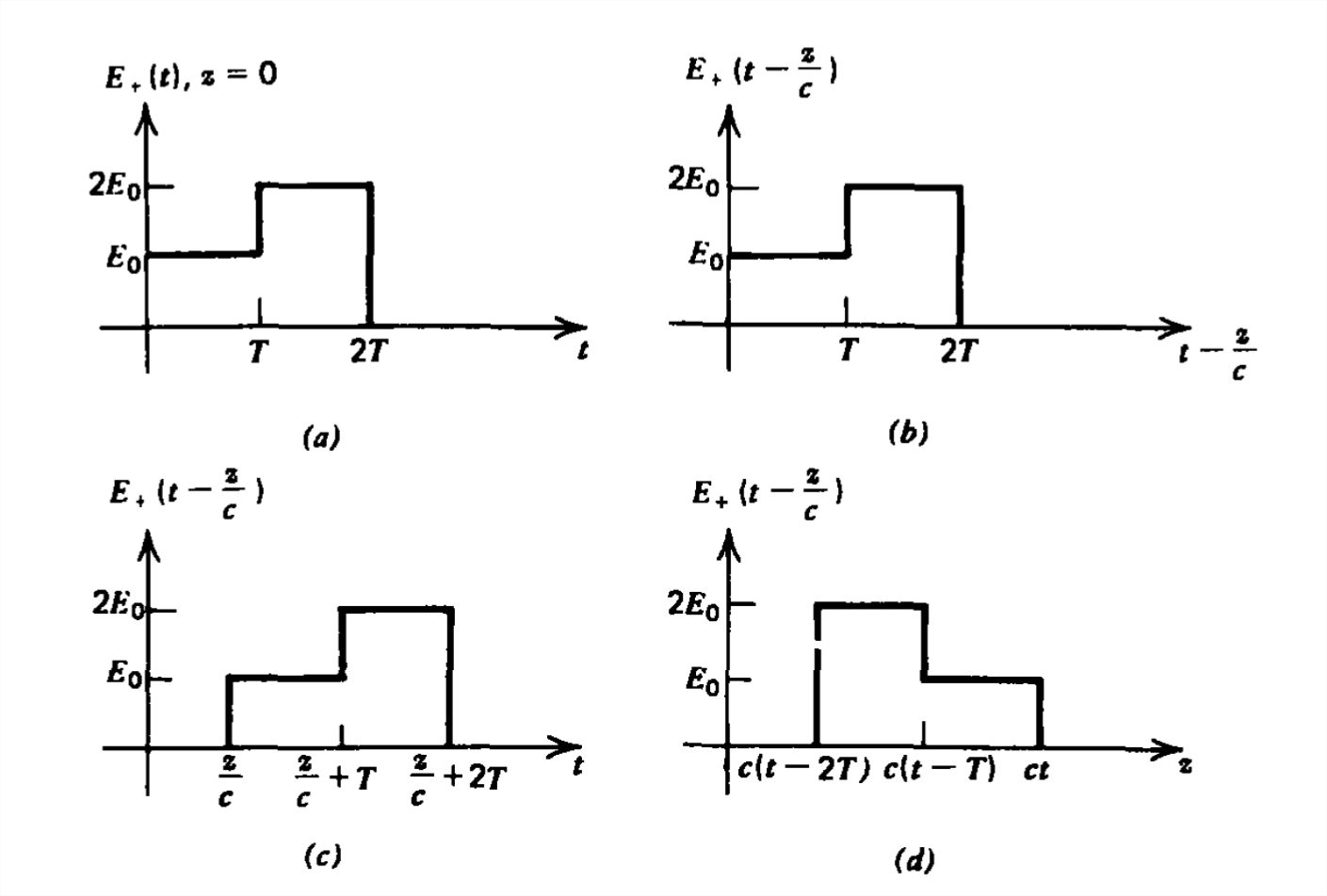
Note that \(z\) can only be positive as causality imposes the condition that time can only be increasing. The response at any positive position \(z\) to an initial \(E_{+}\), pulse imposed at \(z = 0\) has the same shape in time but occurs at a time \(z/c\) later. The pulse travels the distance \(z\) at the speed \(c\). This is why the function \(E_{+}(t -z/c)\) is called a positively traveling wave.

In Figure 7-3d we plot the same function versus \(z\). Its appearance is inverted as that part of the pulse generated first (step of amplitude \(E_{0}\)) will reach any positive position \(z\) first. The second step of amplitude \(2E_{0}\) has not traveled as far since it was generated a time \(T\) later. To help in plotting, we use the same criterion on the argument as used in the plot versus time, only we solve for \(z\). The important rule we use is that as long as the argument of a function remains constant, the value of the function is unchanged, no matter how the individual terms in the argument change.

Thus, as long as

\[ t -z/c= \mathrm{const} \]

\(E_{+}(t -z/c)\) is unchanged. As time increases, so must \(z\) to satisfy (19) at the rate

\[ t-\frac{z}{c}=\mathrm{const}\Rightarrow \frac{\mathrm{d} z}{\mathrm{d} t}=-c \]

to keep the \(E_{+}\), function constant.

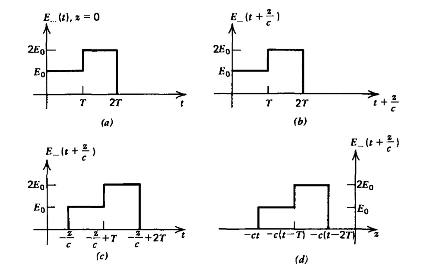
For similar reasons \(E_{+}(t +z/c)\) represents a traveling wave at the speed \(c\) in the negative \(z\) direction as an observer must move to keep the argument \(t +z/c\) constant at speed:

\[ t+\frac{z}{c}=\mathrm{const}\Rightarrow \frac{\mathrm{d} z}{\mathrm{d} t}=c \]

as demonstrated for the same staircase pulse in Figure 7-4. Note in Figure 7-4d that the pulse is not inverted when plotted versus \(z\) as it was for the positively traveling wave, because that part of the pulse generated first (step of amplitude \(E_{0}\)) reaches the maximum distance but in the negative \(z\) direction. These differences between the positively and negatively traveling waves are functionally due to the difference in signs in the arguments \((t -z/c)\) and \((t +z/c)\).

Sources of Plane Waves

These solutions are called plane waves because at any constant \(z\) plane the fields are constant and do not vary with the \(x\) and \(y\) coordinates.

The idealized source of a plane wave is a time varying current sheet of infinite extent that we take to be \(x\) directed,

Figure 7-4 (a) \(E_{-}\left ( t \right )\) at \(z =0\) is a staircase pulse. (b) \(E_{-}\left ( \phi \right )\) always has the same form of (a) when plotted versus \(\phi\). Here \(\phi=t+z/c\). (c) When plotted versus \(t\), the pulse is translated in time where \(z\) must be negative to keep \(t\) positive. (d) When plotted versus \(z\), it is translated but not inverted.

as shown in Figure 7-5. From the boundary condition on the discontinuity of tangential \(\textbf{H}\), we find that the \(x\)-directed current sheet gives rise to a \(y\)-directed magnetic field:

\[ H_{y}\left ( z=0_{+} \right )-H_{y}\left ( z=0_{-} \right )=-K_{x}\left ( t \right ) \]

In general, a uniform current sheet gives rise to a magnetic field perpendicular to the direction of current flow but in the plane of the sheet. Thus to generate an \(x\)-directed magnetic field, a \(y\)-directed surface current is required.

Since there are no other sources, the waves must travel away from the sheet so that the solutions on each side of the sheet are of the form

\[ H_{y}\left ( z,t \right )=\left\{\begin{matrix}
H_{+}\left ( t-z/c \right )\\ 
H_{-}\left ( t+z/c \right )
\end{matrix}\right.\quad E_{x}\left ( z,t \right )=\left\{\begin{matrix}
\eta H_{+}\left ( t-z/c \right ),\quad z>0\\ 
-\eta H_{-}\left ( t+z/c \right ),\quad z<0
\end{matrix}\right. \]

For \(z >0\), the waves propagate only in the positive \(z\) direction. In the absence of any other sources or boundaries, there can be no negatively traveling waves in this region. Similarly for \z <0(\), we only have waves propagating in the \(-z\) direction. In addition to the boundary condition of (22), the tangential component of \(\textbf{E}\) must be continuous across the sheet at \( z =0\)

\[ \left.\begin{matrix}H_{+}\left ( t \right )-H_{-}\left ( t \right )=-K_{x}\left ( t \right )
\\ \eta \left [ H_{+}\left ( t \right )+H_{-}\left ( t \right ) \right ]=0
\end{matrix}\right\}\Rightarrow H_{+}\left ( t \right )=-H_{-}\left ( t \right )=\frac{-K_{x}\left ( t \right )}{2} \]

Figure 7-5 (a) A linearly polarized plane wave is generated by an infinite current sheet. The electric field is in the direction opposite to the current on either side of the sheet. The magnetic field is perpendicular to the current but in the plane of the current sheet and in opposite directions as given by the right-hand rule on either side of the sheet. The power flow \(\textbf{S}\) is thus perpendicular to the current and to the sheet. (b) The field solutions for \(t >2 T\) if the current source is a staircase pulse in time.

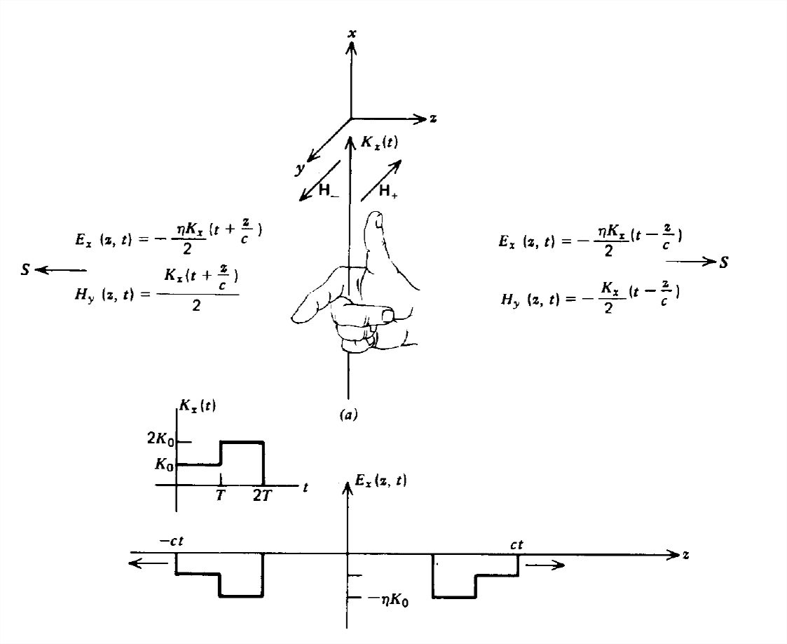
so that the electric and magnetic fields have the same shape as the current. Because the time and space shape of the fields remains unchanged as the waves propagate, linear dielectric media are said to be nondispersive.

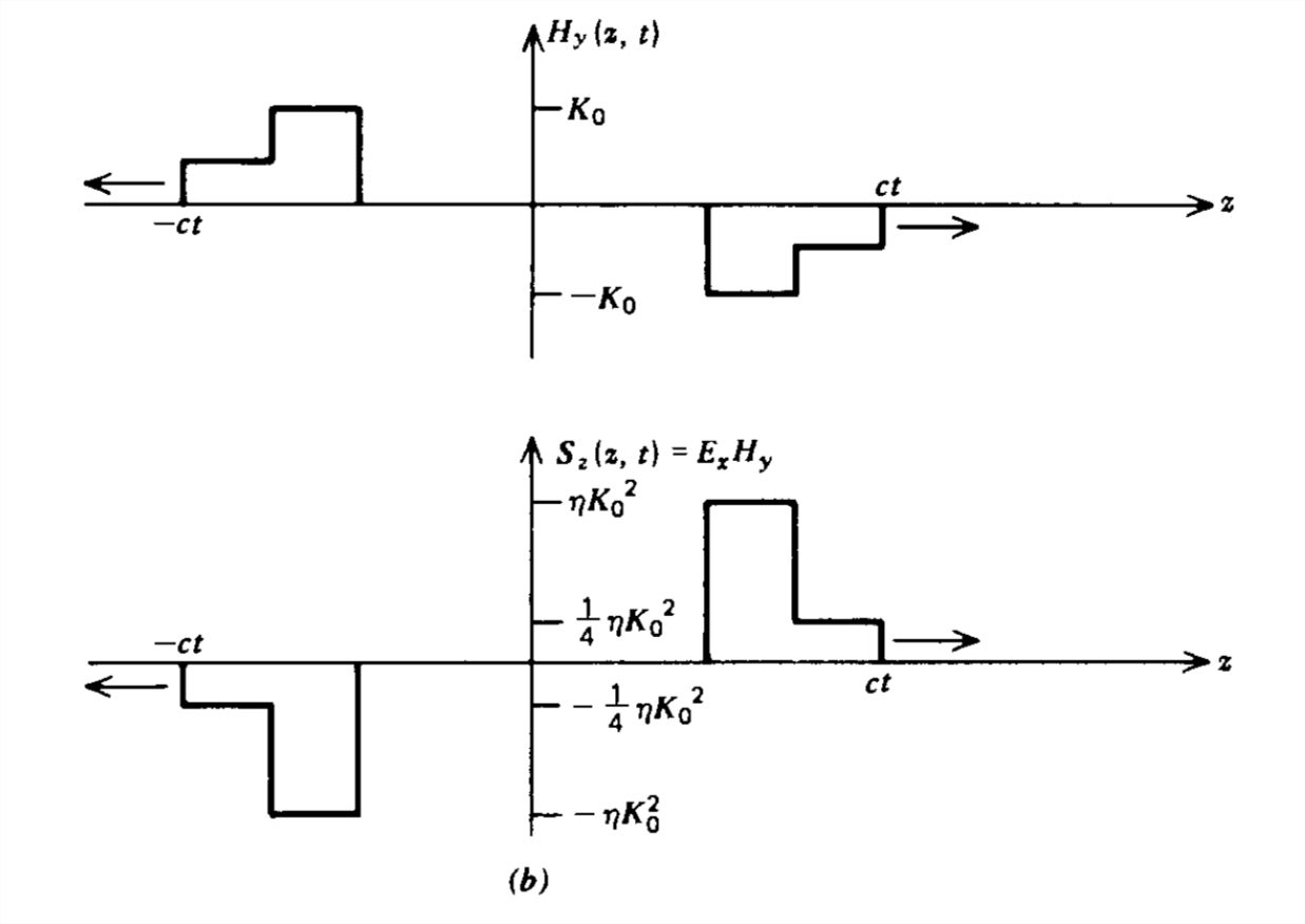
Note that the electric field at \(z =0\) is in the opposite direction as the current, so the power per unit area delivered by the current sheet,

\[ -\textbf{E}\left ( z=0,t \right )\cdot \textbf{K}_{x}\left ( t \right )=\frac{\eta K_{x}^{2}\left ( t \right )}{2} \]

is equally carried away by the Poynting vector on each side of the sheet:

\[ \textbf{S}\left ( z=0 \right )=\textbf{E}\times \textbf{H}=\left\{\begin{matrix}
\frac{\eta K_{x}^{2}\left ( t \right )}{4}\textbf{i}_{x},\quad z> 0\\ 
\frac{-\eta K_{x}^{2}\left ( t \right )}{4},\quad z<0
\end{matrix}\right. \]

A Brief Introduction to the Theory of Relativity

Maxwell's equations show that electromagnetic waves propagate at the speed \(c_{0}=1/\sqrt{\varepsilon_{0}\mu _{0}}\) in vacuum. Our natural intuition would tell us that if we moved at a speed \(v\) we would measure a wave speed of \(c_{0}-v\) when moving in the same direction as the wave, and a speed \(c_{0}+v\) when moving in the opposite direction. However, our intuition would be wrong, for nowhere in the free space, source-free Maxwell's equations does the speed of the observer appear. Maxwell's equations predict that the speed of electromagnetic waves is co for all observers no matter their relative velocity. This assumption is a fundamental postulate of the theory of relativity and has been verified by all experiments. The most notable experiment was performed by A. A. Michelson and E. W. Morley in the late nineteenth century, where they showed that the speed of light reflected between mirrors is the same whether it propagated in the direction parallel or perpendicular to the velocity of the earth. This postulate required a revision of the usual notions of time and distance.

If the surface current sheet of Section 7-3-3 is first turned on at \(t = 0\), the position of the wave front on either side of the sheet at time \(t\) later obeys the equality

\[ z^{2}-c_{0}^{2}t^{2}=0 \]

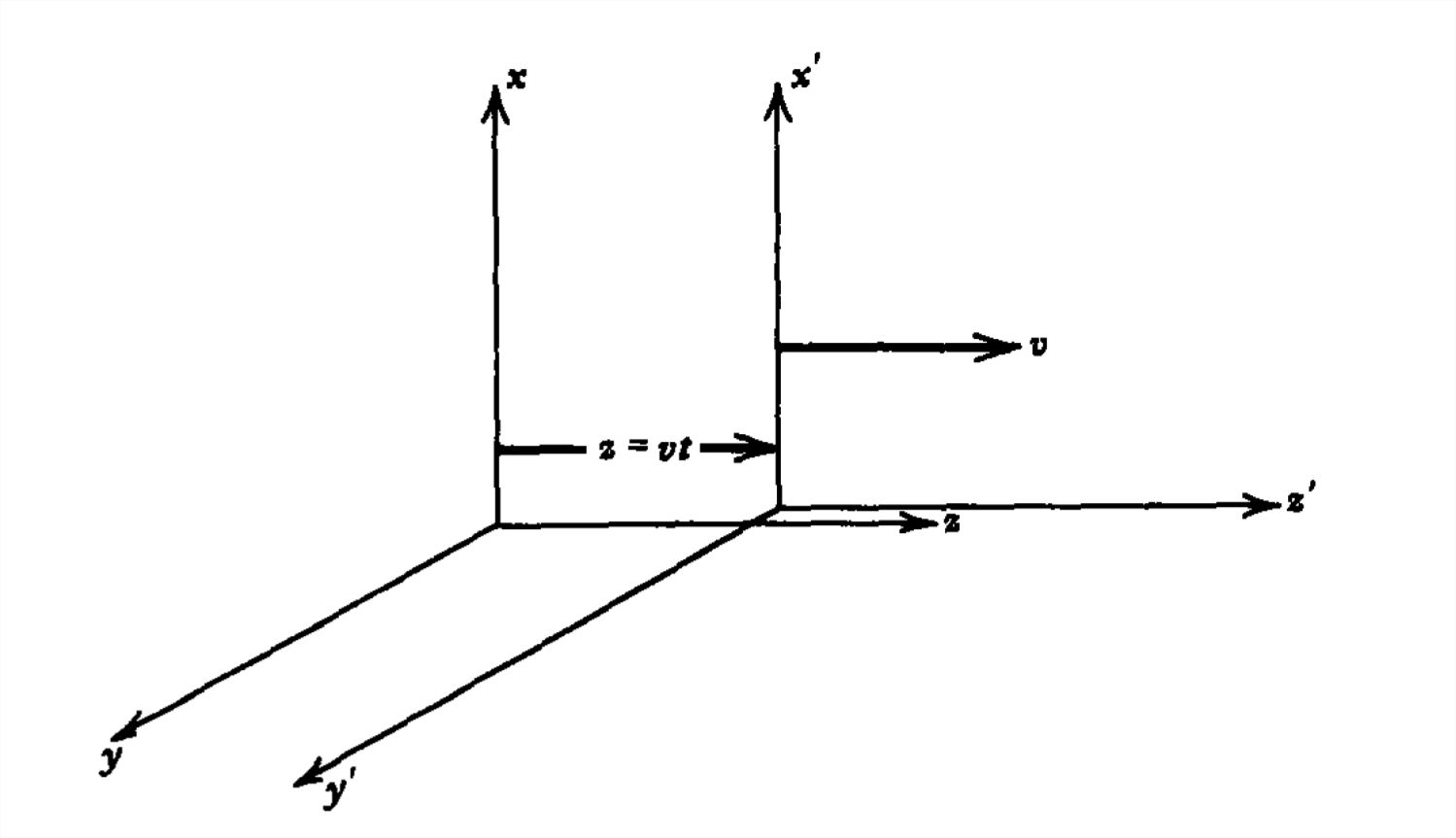
Similarly, an observer in a coordinate system moving with constant velocity \(u\textbf{i}_{z}\), which is aligned with the current sheet at \(t=0\) finds the wavefront position to obey the equality

\[ z'^{2}-c_{0}^{2}t'^{2}=0 \]

The two coordinate systems must be related by a linear transformation of the form

\[ z'=a_{1}z+a_{2}t,\quad t'=b_{1}z+b_{2}t \]

The position of the origin of the moving frame \((z'=0)\) as measured in the stationary frame is \(z = vt\), as shown in Figure 7-6, so that \(a_{1}\) and \(a_{2}\) are related as

\[ 0=a_{1}vt+a_{2}t\Rightarrow a_{1}v+a_{2}=0 \]

We can also equate the two equalities of (27) and (28),

\[ z^{2}-c_{0}^{2}t^{2}=z'^{2}-c_{0}^{2}t'^{2}=\left ( a_{1}z+a_{2}t \right )^{2}-c_{0}^{2}\left ( b_{1}z+b_{2}t \right ) \]

so that combining terms yields

\[ z^{2}\left ( 1-a_{1}^{2}+c_{0}^{2}b_{1}^{2} \right )-c_{0}^{2}t^{2}\left ( 1+\frac{a_{2}^{2}}{c_{0}^{2}}-b_{2}^{2} \right )-2\left ( a_{1}a_{2}-c_{0}^{2}b_{1}b_{2} \right )zt=0 \]

Since (32) must be true for all \(z\) and \(t\), each of the coefficients must be zero, which with (30) gives solutions

\[ a_{1}=\frac{1}{\sqrt{1-\left ( v/c_{0} \right )^{2}}},\quad b_{1}=\frac{-v/c_{0}^{2}}{\sqrt{1-\left ( v/c_{0} \right )^{2}}}\\
   a_{2}=\frac{-v}{\sqrt{1-\left ( v/c_{0} \right )^{2}}},\quad b_{2}=\frac{1}{\sqrt{1-\left ( v/c_{0} \right )^{2}}} \]

Figure 7-6 The primed coordinate system moves at constant velocity \(v\textbf{i}_{z}\), with respect to a stationary coordinate system. The free space speed of an electromagnetic wave is \(c_0\) as measured by observers in either coordinate system no matter the velocity \(v\).

The transformations of (29) are then

\[ z'=\frac{z-vt}{\sqrt{1-\left ( v/c_{0} \right )^{2}}},\quad t'=\frac{t-vz/c_{0}^{2}}{\sqrt{1-\left ( v/c_{0} \right )^{2}}} \]

and are known as the Lorentz transformations. Measured lengths and time intervals are different for observers moving at different speeds. If the velocity \(v\) is much less than the speed of light, (34) reduces to the Galilean transformations,

\[ \lim_{v/c\ll 1}z'\approx z-vt,\quad t'\approx t \]

which describe our usual experiences at nonrelativistic speeds. The coordinates perpendicular to the motion are unaffected by the relative velocity between reference frames

\[ x'=x,\quad y'=y \]

Continued development of the theory of relativity is beyond the scope of this text and is worth a course unto itself. Applying the Lorentz transformation to Newton's law and Maxwell's equations yields new results that at first appearance seem contrary to our experiences because we live in a world where most material velocities are much less than \(c_0\). However, continued experiments on such disparate time and space scales as between atomic physics and astronomics verify the predictions of relativity theory, in part spawned by Maxwell's equations.