7.4: Sinusoidal Time Variations

Frequency and Wavenumber

If the current sheet of Section 7-3-3 varies sinusoidally with time as \(\textrm{Re}\left ( K_{0}e^{j\omega t} \right )\), the wave solutions require the fields to vary as \(e^{j\omega t\left ( t-z/c \right )}\) and \(e^{j\omega t\left ( t+z/c \right )}\).

\[ H_{y}\left ( z,t \right )=\left\{\begin{matrix}
\textrm{Re}\left ( -\frac{K_{0}}{2}e^{j\omega t\left ( t-z/c \right )} \right ),\quad z>0\\ 
\textrm{Re}\left ( +\frac{K_{0}}{2}e^{j\omega t\left ( t+z/c \right )} \right ),\quad z<0
\end{matrix}\right.\\
E_{x}\left ( z,t \right )=\left\{\begin{matrix}
\textrm{Re}\left ( -\frac{\eta K_{0}}{2}e^{j\omega t\left ( t-z/c \right )} \right ),\quad z>0\\ 
\textrm{Re}\left ( +\frac{\eta K_{0}}{2}e^{j\omega t\left ( t+z/c \right )} \right ),\quad z<0
\end{matrix}\right. \]

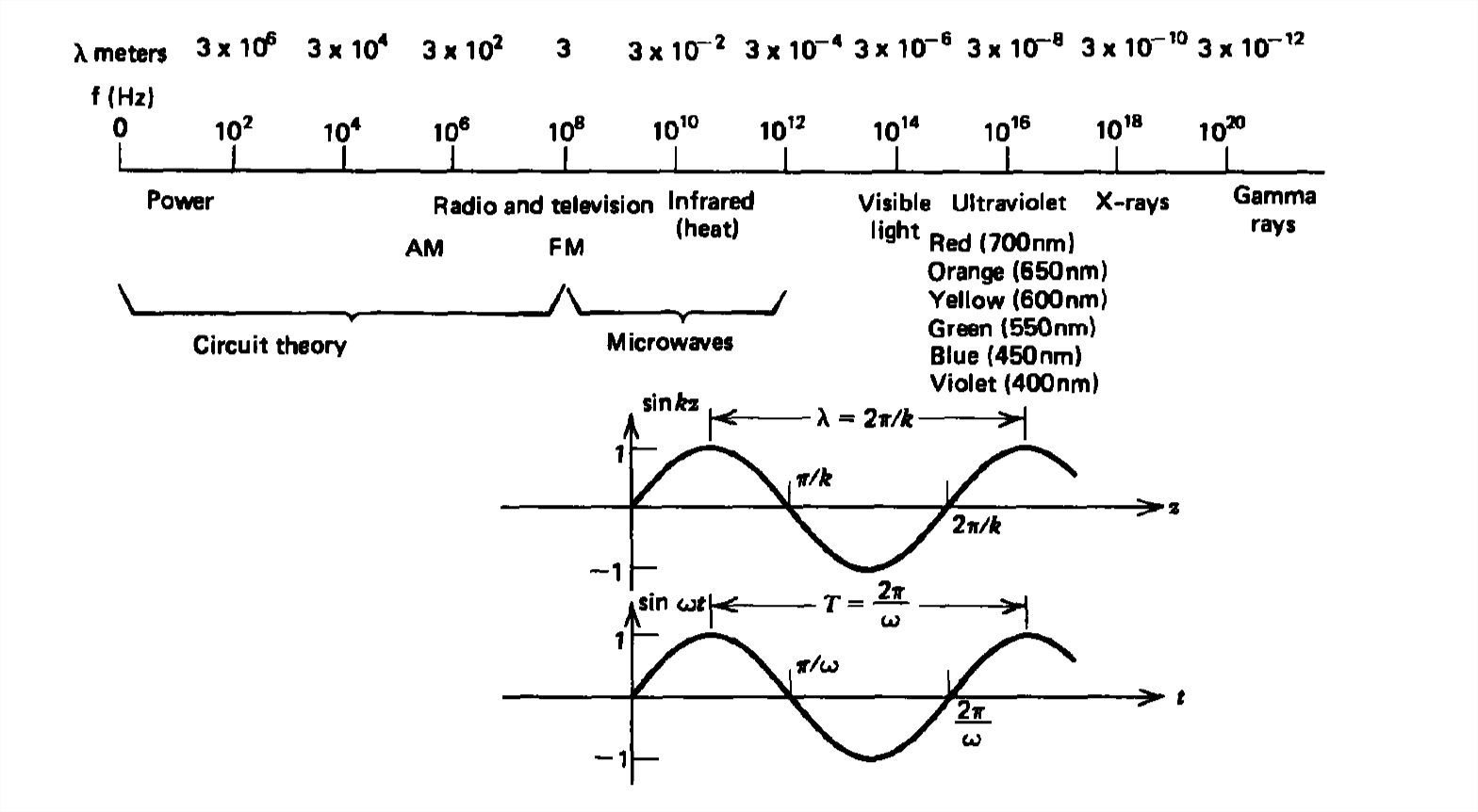
At a fixed time the fields then also vary sinusoidally with position so that it is convenient to define the wavenumber as

\[ k=\frac{2\pi }{\lambda }=\frac{\omega }{c}=\omega \sqrt{\mu \varepsilon } \]

where \(\lambda\) is the fundamental spatial period of the wave. At a fixed position the waveform is also periodic in time with period \(T\):

\[ T=\frac{1}{f}=\frac{2\pi }{\omega } \]

where \(f\) is the frequency of the source. Using (3) with (2) gives us the familiar frequency-wavelength formula:

\[ \omega =kc\Rightarrow f\lambda =c \]

Throughout the electromagnetic spectrum, summarized in Figure 7-7, time-varying phenomena differ only in the scaling of time and size. No matter the frequency or wavelength, although easily encompassing \(20\) orders of magnitude, electromagnetic phenomena are all described by Maxwell's equations. Note that visible light only takes up a tiny fraction of the spectrum.

Figure 7-7 Time-varying electromagnetic phenomena differ only in the scaling of time (frequency) and size (wavelength). In linear dielectric media the frequency and wavelength are related as \( f\lambda =c\left ( \omega =kc \right )\), where \(c=1/\sqrt{\varepsilon \mu }\) is the speed of light in the medium.

For a single sinusoidally varying plane wave, the time-average electric and magnetic energy densities are equal because the electric and magnetic field amplitudes are related through the wave impedance \(\eta \):

\[<\omega _{m}>=<\omega _{\varepsilon }>=\frac{1}{4}\mu \left | \textbf{H} \right |^{2}=\frac{1}{4}\varepsilon  \left | \textbf{E} \right |^{2}=\frac{1}{16}\mu \textbf{K}_{0}^{2} \]

From the complex Poynting theorem derived in Section 7-2-4, we then see that in a lossless region with no sources for \(\left | z \right |>0\) that \(\hat{P_{d}}=0\) so that the complex Poynting vector has zero divergence. With only one-dimensional variations with \(z\), this requires the time-average power density to be a constant throughout space on each side of the current sheet:

\[ \begin{align} <\textbf{S}> & = \frac{1}{2}\textrm{Re}\left [ \hat{\textbf{E}}\left ( \textbf{r} \right )\times \hat{\textbf{H}}^{*}\left ( \textbf{r} \right ) \right ] \\ & = \left\{\begin{matrix} \frac{1}{8}\eta K_{0}^{2}\textbf{i}_{z},\quad z>0\\ -\frac{1}{8}\eta K_{0}^{2}\textbf{i}_{z},\quad z<0 \end{matrix}\right. \nonumber  \end{align}  \]

The discontinuity in \(<\textbf{S}>\) at \(z = 0\) is due to the power output of the source.

Doppler Frequency Shifts

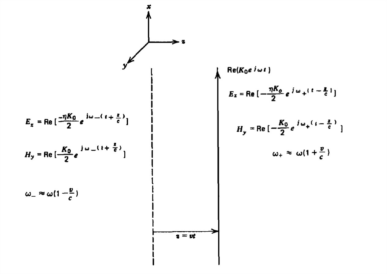
If the sinusoidally varying current sheet \(\textrm{Re}\left ( K_{0}e^{j\omega t} \right ) \) moves with constant velocity \(v\textbf{i}_{z}\), as in Figure 7-8, the boundary conditions are no longer at \(z =0\) but at \(z = vt\). The general form of field solutions are then:

\[ H_{y}\left ( z,t \right )=\left\{\begin{matrix}
\textrm{Re}\left ( \hat{H}_{+}e^{j\omega_{+}\left ( t-z/c \right )} \right ),\quad z>vt\\ 
\textrm{Re}\left ( \hat{H}_{-}e^{j\omega_{-}\left ( t+z/c \right )} \right ),\quad z<vt
\end{matrix}\right.\\
E_{x}\left ( z,t \right )=\left\{\begin{matrix}
\textrm{Re}\left ( \eta \hat{H}_{+}e^{j\omega_{+}\left ( t-z/c \right )} \right ),\quad z>vt\\ 
\textrm{Re}\left ( -\eta \hat{H}_{-}e^{j\omega_{-}\left ( t+z/c \right )} \right ),\quad z<vt
\end{matrix}\right.  \]

where the frequencies of the fields \(\omega_{+}\) and \(\omega_{-}\) on each side of the sheet will be different from each other as well as differing from the frequency of the current source \(\omega\). We assume \(v/c\ll 1\) so that we can neglect relativistic effects discussed in Section 7-3-4. The boundary conditions

\[ E_{x+}\left ( z=vt \right )=E_{x-}\left ( z=vt \right )\Rightarrow \hat{H}_{+}e^{j\omega_{+}t\left ( 1-v/c \right ) }=-\hat{H}_{-}e^{j\omega_{+}t\left ( 1+v/c \right ) }\\
H_{y+}\left ( z=vt \right )-H_{y-}\left ( z=vt \right )=-K_{x}\\
\Rightarrow \hat{H}_{+}e^{j\omega_{+}t\left ( 1-v/c \right ) }-\hat{H}_{-}e^{j\omega_{+}t\left ( 1+v/c \right ) }=-K_{0}e^{j\omega t} \]

must be satisfied for all values of \(t\) so that the exponential time factors in (8) must all be equal, which gives the shifted

Figure 7-8 When a source of electromagnetic waves moves towards an observer, the frequency is raised while it is lowered when it moves away from an observer.

frequencies on each side of the sheet as

\[ \omega_{+}=\frac{\omega }{1-v/c}\approx \omega \left ( 1+\frac{v}{c} \right ),\\
\omega_{-}=\frac{\omega }{1+v/c}\approx \omega \left ( 1-\frac{v}{c} \right )\Rightarrow \hat{H}_{+}=-\hat{H}_{-}=-\frac{K_{0}}{2} \]

where \(v/c\ll 1\). When the source is moving towards an observer, the frequency is raised while it is lowered when it moves away. Such frequency changes due to the motion of a source or observer are called Doppler shifts and are used to measure the velocities of moving bodies in radar systems. For \(v/c\ll 1\), the frequency shifts are a small percentage of the driving frequency, but in absolute terms can be large enough to be easily measured. At a velocity \(v=300\, \textrm{m/sec}\) with a driving frequency of \(f=10^{10}\, \textrm{Hz}\), the frequency is raised and lowered on each side of the sheet by \(\Delta f=\pm f\left ( v/c \right )=\pm 10^{4} \, \textrm{Hz}\).

Ohmic Losses

Thus far we have only considered lossless materials. If the medium also has an Ohmic conductivity \(\sigma \), the electric field will cause a current flow that must be included in Ampere's law:

\[ \frac{\partial E_{x}}{\partial z}=-\mu \frac{\partial H_{y}}{\partial t}\\
\frac{\partial H_{y}}{\partial z}=-J_{x}-\varepsilon \frac{\partial E_{x}}{\partial t}=-\sigma E_{x}-\varepsilon \frac{\partial E_{x}}{\partial t} \]

where for conciseness we only consider the \(x\)-directed electric field solution as the same results hold for the \(E_{y}\), \(H_{x}\) solution. Our wave solutions of Section 7-3-2 no longer hold with this additional term, but because Maxwell's equations are linear with constant coefficients, for sinusoidal time variations the solutions in space must also be exponential functions, which we write as

\[ E_{x}\left ( z,t \right )=\textrm{Re}\left ( \hat{E}_{0}\,e^{j\left ( \omega t-kz \right )} \right )\\
H_{y}\left ( z,t \right )=\textrm{Re}\left ( \hat{H}_{0}\,e^{j\left ( \omega t-kz \right )} \right ) \]

where \(\hat{E}_{0}\) and \(\hat{H}_{0}\) are complex amplitudes and the wavenumber \(k\) is no longer simply related to \(\omega\) as in (4) but is found by substituting (11) back into (10):

\[ -jk\hat{E}_{0}=-j\omega \mu \hat{H}_{0}\\-jk\hat{H}_{0}=-j\omega \varepsilon \left ( 1+\sigma /j\omega \varepsilon  \right ) \hat{E}_{0} \]

This last relation was written in a way that shows that the conductivity enters in the same way as the permittivity so that we can define a complex permittivity \(\hat{\varepsilon }\) as

\[ \hat{\varepsilon }=\varepsilon \left ( 1+\sigma /j\omega \varepsilon  \right ) \]

Then the solutions to (12) are

\[ \frac{\hat{E}_{0}}{\hat{H}_{0}}=\frac{\omega \mu }{k}=\frac{k}{\omega \hat{\varepsilon }}\Rightarrow k^{2}= \omega ^{2}\mu \hat{\varepsilon }= \omega ^{2}\mu\varepsilon \left ( 1+\frac{\sigma }{j\omega \varepsilon } \right ) \]

which is similar in form to (2) with a complex permittivity.

There are two interesting limits of (14):

(a) Low Loss Limit

If the conductivity is small so that \(\sigma /\omega \varepsilon \ll 1\), then the solution of (14) reduces to

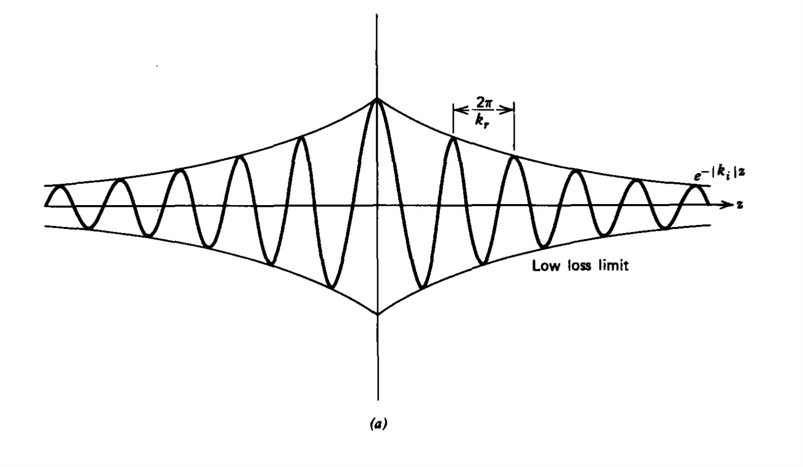
\[ \lim_{\sigma /\omega \varepsilon \ll 1}k=\pm \omega \sqrt{\mu \varepsilon }\left ( 1+\frac{\sigma }{2j\omega \varepsilon } \right )=\pm \left ( \frac{\omega }{c}-\frac{j\sigma }{2}\sqrt{\frac{\mu }{\varepsilon }} \right ) \]

where \(c\) is the speed of the light in the medium if there were no losses, \(c=1/\sqrt{\mu \varepsilon }\). Because of the spatial exponential dependence in (11), the real part of \(k\) is the same as for the lossless case and represents the sinusoidal spatial distribution of the fields. The imaginary part of \(k\) represents the exponential decay of the fields due to the Ohmic losses with exponential decay length \(\frac{1}{2}\sigma \eta \), where \(\eta =\sqrt{\mu /\varepsilon }\) is the wave impedance. Note that for waves traveling in the positive \(z\) direction we take the upper positive sign in (15) using the lower negative sign for negatively traveling waves so that the solutions all decay and do not grow for distances far from the source. This solution is only valid for small \(\sigma \) so that the wave is only slightly damped as it propagates, as illustrated in Figure 7-9a.

Figure 7-9 (a) In a slightly lossy dielectric, the fields decay away from a source at a slow rate while the wavelength is essentially unchanged. (b) In the large loss limit the spatial decay rate is equal to the skin depth. The wavelength also equals the skin depth.

(b) Large Loss Limit

In the other extreme of a highly conducting material so that \(\sigma /\omega \varepsilon \gg 1\), (14) reduces to

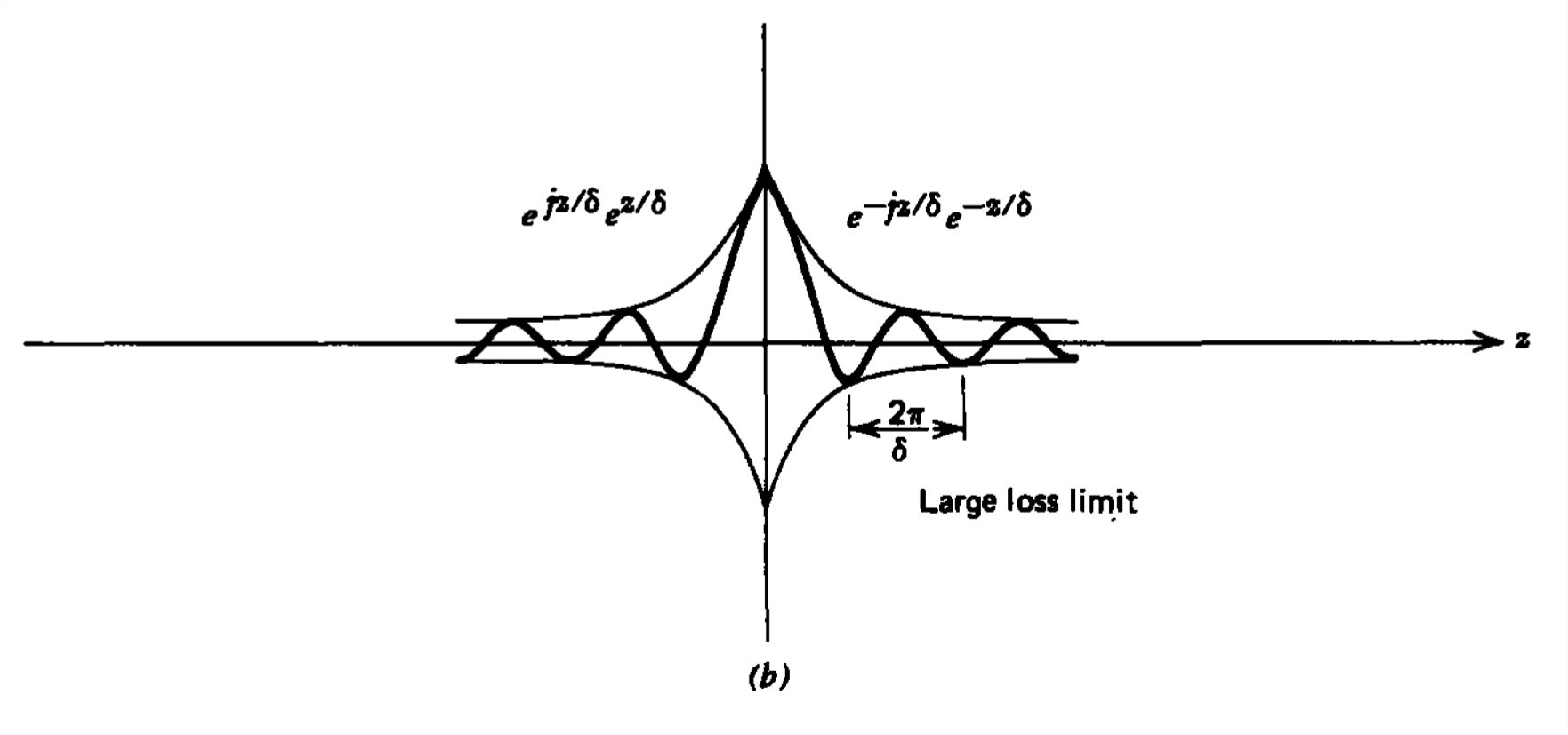
\[ \lim_{\sigma /\omega \varepsilon \gg 1}k^{2}\approx -j\omega \mu \sigma \Rightarrow k=\pm \frac{1-j}{\delta },\quad \delta =\sqrt{\frac{2}{\omega \mu \sigma }} \]

where \(\delta \) is just the skin depth found in Section 6-4-3 for magneto-quasi-static fields within a conductor. The skin-depth term also arises for electrodynamic fields because the large loss limit has negligible displacement current compared to the conduction currents.

Because the real and imaginary part of \(k\) have equal magnitudes, the spatial decay rate is large so that within a few oscillation intervals the fields are negligibly small, as illustrated in Figure 7-9b. For a metal like copper with \(\mu =\mu _{0}=4\pi \times 10^{-7} \, \textrm{henry/m}\) and \(\sigma \approx 6\times 10^{7}\,\textrm{siemens/m}\) at a frequency of \(1\,\textrm{MHz}\), the skin depth is \(\delta \approx 6.5\times 10^{-5}\,\textrm{m}\).

High-Frequency Wave Propagation in Media

Ohm's law is only valid for frequencies much below the collision frequencies of the charge carriers, which is typically on the order of \(10^{13}\,\textrm{Hz}\). In this low-frequency regime the inertia of the particles is negligible. For frequencies much higher than the collision frequency the inertia dominates and the current constitutive law for a single species of charge carrier \(q\) with mass \(m\) and number density \(n\) is as found in Section 3-2-2d:

\[ \partial \textbf{J}_{f}/\partial t=\omega_{p} ^{2}\varepsilon \textbf{E} \]

where \(\omega_{p}=\sqrt{q^{2}n/m\varepsilon }\) is the plasma frequency. This constitutive law is accurate for radio waves propagating in the ionosphere, for light waves propagating in many dielectrics, and is also valid for superconductors where the collision frequency is zero.

Using (17) rather than Ohm's law in (10) for sinusoidal time and space variations as given in (11), Maxwell's equations are

\[ \frac{\partial E_{x}}{\partial z}=-\mu \frac{\partial H_{y}}{\partial t}\Rightarrow -jk\hat{E}_{0}=-j\omega \mu \hat{H}_{0}\\
\frac{\partial H_{y}}{\partial z}=-J_{x}-\varepsilon \frac{\partial E_{x}}{\partial t}\Rightarrow -jk\hat{H}_{0}=-j\omega \varepsilon \left ( 1-\frac{\omega_{p}^{2}}{\omega ^{2}} \right ) \hat{E}_{0} \]

The effective permittivity is now frequency dependent:

\[ \hat{\varepsilon }=\varepsilon \left ( 1-\omega_{p}^{2}/\omega^{2} \right ) \]

The solutions to (18) are

\[ \frac{\hat{E}_{0}}{\hat{H}_{0}}=\frac{\omega \mu }{k}=\frac{k}{\omega \hat{\varepsilon }}\Rightarrow k^{2}= \omega ^{2}\mu \hat{\varepsilon }= \frac{\omega ^{2}-\omega _{p}^{2}}{c^{2}} \]

For \(\omega >\omega_{p}\), \(k\) is real and we have pure propagation where the wavenumber depends on the frequency. For \(\omega <\omega_{p}\), \(k\) is imaginary representing pure exponential decay.

Poynting's theorem for this medium is

\[ \begin{align} \nabla\cdot \textbf{S}+\frac{\partial }{\partial t}\left ( \frac{1}{2}\varepsilon \left | \textbf{E} \right |^{2}+\frac{1}{2}\mu \left | \textbf{H} \right |^{2} \right )& =-\textbf{E}\cdot \textbf{J}_{f} =-\frac{1}{\omega _{p}^{2}\varepsilon }\textbf{J}_{f}\cdot \frac{\partial \textbf{J}_{f}}{\partial t} \\ & =-\frac{\partial }{\partial t}\left ( \frac{1}{\omega _{p}^{2}\varepsilon }\frac{\left | \textbf{J}_{f} \right |^{2}}{2} \right ) \nonumber  \end{align}  \]

Because this system is lossless, the right-hand side of (21) can be brought to the left-hand side and lumped with the energy densities:

\[ \nabla\cdot \textbf{S}+\frac{\partial }{\partial t}\left [ \frac{1}{2}\varepsilon \left | \textbf{E} \right |^{2}+\frac{1}{2}\mu \left | \textbf{H} \right |^{2}+\frac{1}{2}\frac{1}{\omega _{p}^{2}\varepsilon }\left | \textbf{J}_{f} \right |^{2}  \right ] =0  \]

This new energy term just represents the kinetic energy density of the charge carriers since their velocity is related to the current density as

\[ \textbf{J}_{f}=qn\textbf{v}\Rightarrow \frac{1}{2}\frac{1}{\omega _{p}^{2}\varepsilon }\left | \textbf{J}_{f} \right |^{2}=\frac{1}{2}mn\left |\textbf{v}  \right |^{2} \]

Dispersive Media

When the wavenumber is not proportional to the frequency of the wave, the medium is said to be dispersive. A nonsinusoidal time signal (such as a square wave) will change shape and become distorted as the wave propagates because each Fourier component of the signal travels at a different speed.

To be specific, consider a stationary current sheet source at \(z =0\) composed of two signals with slightly different frequencies:

\[\] \[ \begin{aligned}
K(t) & =K_0\left[\cos \left(\omega_0+\Delta \omega\right) t+\cos \left(\omega_0-\Delta \omega\right) t\right] \\
& =2 K_0 \cos \Delta \omega t \cos \omega_0 t
\nonumber \end{aligned} \]

With \(\Delta \omega \ll \omega \) the fast oscillations at frequency \(\omega_0\) are modulated by the slow envelope function at frequency \(\Delta \omega\). In a linear dielectric medium this wave packet would propagate away from the current sheet at the speed of light, \(c=1/\sqrt{\varepsilon \mu }\)). If the medium is dispersive, with the wavenumber \(k\left ( \omega  \right )\) being a function of \(\omega\), each frequency component in (24) travels at a slightly different speed. Since each frequency is very close to \(\omega_0\) we expand \(k\left ( \omega  \right )\) as

\[ k\left ( \omega_{0}+\Delta \omega   \right )\approx k\left ( \omega_{0} \right )+\frac{\mathrm{d} k}{\mathrm{d} \omega }\Big|_{\omega _{0}}\Delta \omega \\
k\left ( \omega_{0}-\Delta \omega   \right )\approx k\left ( \omega_{0} \right )-\frac{\mathrm{d} k}{\mathrm{d} \omega }\Big|_{\omega _{0}}\Delta \omega  \]

where for propagation \(k\left ( \omega_{0} \right )\) must be real.

The fields for waves propagating in the \(+z\) direction are then of the following form:

\[ \begin{align} E_{x}\left ( z,t \right )& =\textrm{Re}\,\hat{E}_{0}\left ( \textrm{exp}\left \{ j\left [ \left ( \omega_{0}+\Delta \omega  \right )t-\left ( k\left ( \omega _{0} \right )+\frac{dk}{d\omega }\Big|_{\omega _{0}}\Delta \omega  \right )z \right ] \right \} +\textrm{exp}\left \{ j\left [ \left ( \omega_{0}-\Delta \omega  \right )t-\left ( k\left ( \omega _{0} \right )-\frac{dk}{d\omega }\Big|_{\omega _{0}}\Delta \omega  \right )z \right ] \right \}\right ) \\ &
=\textrm{Re}\,\left ( \hat{E}_{0}\, \textrm{exp}\left \{ j\left [ \omega _{0}t-k\left ( \omega _{0} \right ) z\right ] \right \}\left \{ \textrm{exp}\left [ j\Delta \omega \left ( t-\frac{\mathrm{d} k}{\mathrm{d} \omega }\Big|_{\omega _{0}} z\right ) \right ] +\textrm{exp}\left [ -j\Delta \omega \left ( t-\frac{\mathrm{d} k}{\mathrm{d} \omega }\Big|_{\omega _{0}} z \right ) \right ]\right \} \right ) \nonumber \\ &
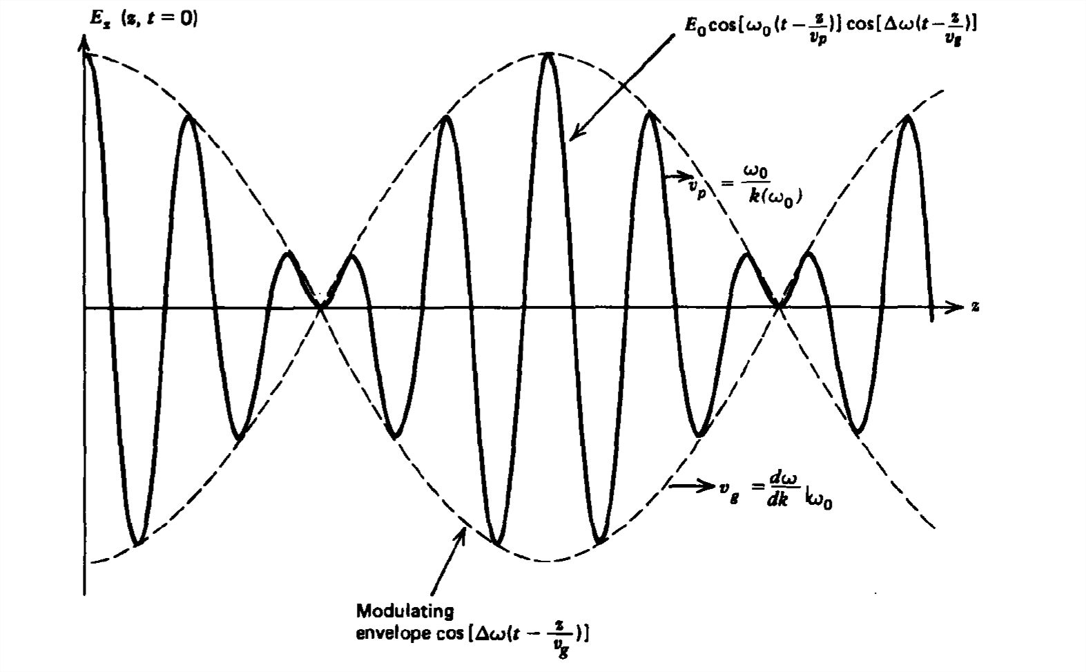
=2E_{0}\cos \left ( \omega _{0}t-k\left ( \omega _{0} \right )z \right )\cos\Delta \omega \left ( t-\frac{\mathrm{d} k}{\mathrm{d} \omega }\Big|_{\omega _{0}} z\right ) \nonumber  \end{align} \]

where without loss of generality we assume in the last relation that \(\hat{E}_{0}=E_{0}\) is real. This result is plotted in Figure 7-10 as a function of \(z\) for fixed time. The fast waves with argument \(\omega_{0}t-k\left ( \omega _{0} \right )z\) travel at the phase speed \(v_{p}=\omega _{0}/k\left ( \omega _{0} \right )\) through the modulating envelope with argument \(\Delta \omega \left ( t-dk/d\omega \big|_{\omega _{0}} z\right )\). This envelope itself travels at the slow speed

\[ t-\frac{\mathrm{d} k}{\mathrm{d} \omega }\Big|_{\omega _{0}}z=\textrm{const}\Rightarrow \frac{\mathrm{d} z}{\mathrm{d} t}=v_{g}=\frac{\mathrm{d} \omega }{\mathrm{d} k}\Big|_{\omega _{0}} \]

known as the group velocity, for it is the velocity at which a packet of waves within a narrow frequency band around \(\omega _{0}\) will travel.

For linear media the group and phase velocities are equal:

\[ \omega =kc\Rightarrow v_{p}=\frac{\omega }{k}=c\\
v_{g}=\frac{\mathrm{d} \omega }{\mathrm{d} k}=c \]

Figure 7-10 In a dispersive medium the shape of the waves becomes distorted so the velocity of a wave is not uniquely defined. For a group of signals within a narrow frequency band the modulating envelope travels at the group velocity \(v_{g}\). The signal within the envelope propagates through at the phase velocity \(v_{p}\).

while from Section 7-4-4 in the high-frequency limit for conductors, we see that

\[ \omega^{2} =k^{2}c^{2}+\omega _{p}^{2}\Rightarrow v_{p}=\frac{\omega }{k}\\
v_{g}=\frac{\mathrm{d} \omega }{\mathrm{d} k}=\frac{k}{\omega }c^{2} \]

where the velocities only make sense when \(k\) is real so that \(\omega > \omega _{p}\). Note that in this limit

\[ v_{g}v_{p}=c^2 \]

Group velocity only has meaning in a dispersive medium when the signals of interest are clustered over a narrow frequency range so that the slope defined by (27), is approximately constant and real.

Polarization

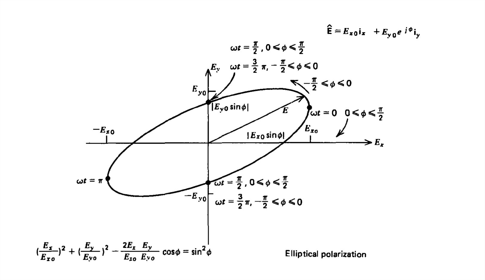
The two independent sets of solutions of Section 7-3-1 both have their power flow \(\textbf{S}=\textbf{E}\times \textbf{H}\) in the \(z\) direction. One solution is said to have its electric field polarized in the \(x\) direction while the second has its electric field polarized in the \(y\) direction. Each solution alone is said to be linearly polarized because the electric field always points in the same direction for all time. If both field solutions are present, the direction of net electric field varies with time. In particular, let us say that the \(x\) and \(y\) components of electric field at any value of \(z\) differ in phase by angle \(\phi \):

\[ \textbf{E}=\textrm{Re}\left [ E_{x_{0}}\textbf{i}_{x}+E_{y_{0}}e^{j\phi }\textbf{i}_{y} \right ]e^{j\omega t}=E_{x_{0}}\cos \omega t\textbf{i}_{x}+E_{y_{0}}\cos \left ( \omega t+\phi  \right )\textbf{i}_{y} \]

We can eliminate time as a parameter, realizing from (31) that

\[ \cos \omega t=E_{x}/E_{x_{0}}\\
\sin\omega t=\frac{\cos\omega t\cos \phi -E_{y}/E_{y_{0}}}{\sin \phi }=\frac{\left ( E_{x}/E_{x_{0}} \right )\cos \phi -E_{y}/E_{y_{0}}}{\sin \phi } \]

and using the identity that

\[ \sin^{2}\omega t+\cos^{2}\omega t \\
=1=\left ( \frac{E_{x}}{E_{x_{0}}} \right )^{2}+\frac{\left ( E_{x}/E_{x_{0}} \right )^{2}\cos^{2}\phi +\left ( E_{y}/E_{y_{0}} \right )^{2}-\left ( 2E_{x}E_{y}/E_{x_{0}}E_{y_{0}} \right )\cos \phi }{\sin^{2} \phi }  \]

to give us the equation of an ellipse relating \(E_{x}\) to \(E_{y}\):

\[ \left ( \frac{E_{x}}{E_{x_{0}}} \right )^{2}+\left ( \frac{E_{y}}{E_{y_{0}}} \right )^{2}-\frac{2E_{x}E_{y}}{E_{x_{0}}E_{y_{0}}}\cos \phi =\sin^{2}\phi  \]

as plotted in Figure 7-1 a. As time increases the electric field vector traces out an ellipse each period so this general case of the superposition of two linear polarizations with arbitrary phase \(\phi\) is known as elliptical polarization. There are two important special cases:

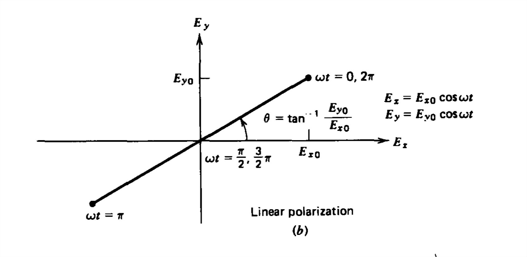
(a) Linear Polarization

If \(E_{x}\) and \(E_{y}\) are in phase so that \(\phi=0\), (34) reduces to

\[ \left ( \frac{E_{x}}{E_{x_{0}}} -\frac{E_{y}}{E_{y_{0}}}\right )^{2}=0\Rightarrow \tan \theta = \frac{E_{y}}{E_{x}}=\frac{E_{y_{0}}}{E_{x_{0}}} \]

The electric field at all times is at a constant angle \( \theta\) to the \(x\) axis. The electric field amplitude oscillates with time along this line, as in Figure 7-11 b. Because its direction is always along the same line, the electric field is linearly polarized.

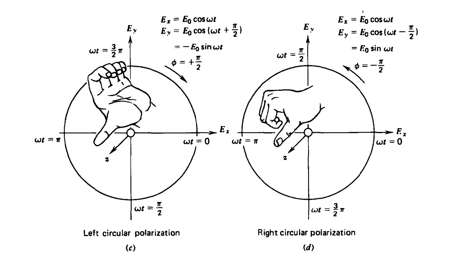
(b) Circular Polarization

If both components have equal amplitudes but are \(90^{\circ}\) out of phase,

\[ E_{x_{0}}=E_{y_{0}}\equiv E_{0},\quad \phi = \pm \pi /2 \]

(34) reduces to the equation of a circle:

\[ E_{x}^{2}+E_{y}^{2}=E_{0}^{2} \]

The tip of the electric field vector traces out a circle as time evolves over a period, as in Figure 7-11c. For the upper (+) sign for \(\phi\) in (36), the electric field rotates clockwise while the negative sign has the electric field rotating counterclockwise. These cases are, respectively, called left and right circular polarization for waves propagating in the \(+z\) direction as found by placing the thumb of either hand in the direction of power flow. The fingers on the left hand curl in the direction of the rotating field for left circular polarization, while the fingers of the right hand curl in the direction of the rotating field for right circular polarization. Left and right circular polarizations reverse for waves traveling in the \(-z\) direction.

Figure 7-11 (a) Two perpendicular field components with phase difference \(\phi\) have the tip of the net electric field vector tracing out an ellipse each period. (b) If both field components are in phase, the ellipse reduces to a straight line. (c) If the field components have the same magnitude but are \(90^{\circ}\) out of phase, the ellipse becomes a circle. The polarization is left circularly polarized to \(z\)-directed power flow if the electric field rotates clockwise and is (d) right circularly polarized if it rotates counterclockwise.

Wave Propagation in Anisotropic Media

Many properties of plane waves have particular applications to optics. Because visible light has a wavelength on the order of \(500 \,\textrm{nm}\), even a pencil beam of light \(1 \,\textrm{mm}\) wide is \(2000\) wavelengths wide and thus approximates a plane wave.

Figure 7-11

(a) Polarizers

Light is produced by oscillating molecules whether in a light bulb or by the sun. This natural light is usually unpolarized as each molecule oscillates in time and direction independent of its neighbors so that even though the power flow may be in a single direction the electric field phase changes randomly with time and the source is said to be incoherent. Lasers, an acronym for "light amplification by stimulated emission of radiation," emits coherent light by having all the oscillating molecules emit in time phase.

A polarizer will only pass those electric field components aligned with the polarizer's transmission axis so that the transmitted light is linearly polarized. Polarizers are made of such crystals as tourmaline, which exhibit dichroism-the selective absorption of the polarization along a crystal axis. The polarization perpendicular to this axis is transmitted.

Because tourmaline polarizers are expensive, fragile, and of small size, improved low cost and sturdy sheet polarizers were developed by embedding long needle-like crystals or chainlike molecules in a plastic sheet. The electric field component in the long direction of the molecules or crystals is strongly absorbed while the perpendicular component of the electric field is passed.

For an electric field of magnitude \(E_0\) at angle \(\phi\) to the transmission axis of a polarizer, the magnitude of the transmitted field is

\[ E_{t}=E_{0}\cos \phi  \]

so that the time-average power flux density is

\[ \begin{align} <S>&=\left | \frac{1}{2}\textrm{Re}\left [ \hat{\textbf{E}}\left ( r \right )\times\hat{\textbf{H}}^{\ast }\left ( r \right )  \right ] \right | \\ &=\frac{1}{2}\frac{E_{0}^{2}}{\eta }\cos ^{2}\phi \nonumber \end{align} \]

which is known as the law of Malus.

(b) Double Refraction (Birefringence)

If a second polarizer, now called the analyzer, is placed parallel to the first but with its transmission axis at right angles, as in Figure 7-12, no light is transmitted. The combination is called a polariscope. However, if an anisotropic crystal is inserted between the polarizer and analyzer, light is transmitted through the analyzer. In these doubly refracting crystals, light polarized along the optic axis travels at speed \(c_{\parallel } \) while light polarized perpendicular to the axis travels at a slightly different speed \(c_{\perp } \). The crystal is said to be birefringent. If linearly polarized light is incident at \(45^{\circ }\) to the axis,

\[ \textbf{E}\left ( z=0,t \right )=E_{0}\left ( \textbf{i}_{x}+\textbf{i}_{y} \right )\textrm{Re}\left ( e^{j\omega t} \right ) \]

the components of electric field along and perpendicular to the axis travel at different speeds:

\[ E_{x}\left ( z,t \right )=E_{0}\,\textrm{Re}\left ( e^{j\left (\omega t-k_{\parallel}z \right )}\right ),\quad k_{\parallel}=\omega /c_{\parallel }\\
E_{y}\left ( z,t \right )=E_{0}\,\textrm{Re}\left ( e^{j\left (\omega t-k_{\perp }z \right )}\right ),\quad k_{\perp }=\omega /c_{\perp } \]

After exiting the crystal at \(z=l\), the total electric field is

\[ \begin{align} \textbf{E}\left ( z=l,t \right )& =E_{0}\,\textrm{Re}\left [ e^{j\omega t}\left ( e^{-jk_{\parallel }l}\textbf{i}_{x}+e^{-jk_{\perp }l}\textbf{i}_{y} \right ) \right ] \\ &
=E_{0}\,\textrm{Re}\left [ e^{j\left (\omega t - k_{\parallel }l\right )}\left ( \textbf{i}_{x}+e^{j\left (k_{\parallel } - k_{\perp }\right )l}\textbf{i}_{y} \right ) \right ] \nonumber \end{align} \]

Figure 7-12 When a linearly polarized wave passes through a doubly refracting (birefringent) medium at an angle to the crystal axes, the transmitted light is elliptically polarized.

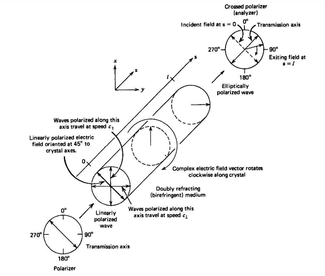
which is of the form of (31) for an elliptically polarized wave where the phase difference is

\[ \phi =\left ( k_{\parallel } -k_{\perp } \right )l=\omega l\left ( \frac{1}{c_{\parallel }}- \frac{1}{c_{\perp }}\right ) \]

When \(\phi\) is an integer multiple of \(2\pi \), the light exiting the crystal is the same as if the crystal were not there so that it is not transmitted through the analyzer. If \(\phi\) is an odd integer multiple of \(\pi\), the exiting light is also linearly polarized but perpendicularly to the incident light so that it is polarized in the same direction as the transmission axis of the analyzer, and thus is transmitted. Such elements are called half-wave plates at the frequency of operation. When \(\phi\) is an odd integer multiple of \(\pi/2\), the exiting light is circularly polarized and the crystal serves as a quarter-wave plate. However, only that polarization of light along the transmission axis of the analyzer is transmitted.

Double refraction occurs naturally in many crystals due to their anisotropic molecular structure. Many plastics and glasses that are generally isotropic have induced birefringence when mechanically stressed. When placed within a polariscope the photoelastic stress patterns can be seen. Some liquids, notably nitrobenzene, also become birefringent when stressed by large electric fields. This phenomena is called the Kerr effect. Electro-optical measurements allow electric field mapping in the dielectric between high voltage stressed electrodes, useful in the study of high voltage conduction and breakdown phenomena. The Kerr effect is also used as a light switch in high-speed shutters. A parallel plate capacitor is placed within a polariscope so that in the absence of voltage no light is transmitted. When the voltage is increased the light is transmitted, being a maximum when \(\phi=\pi\). (See problem 17.)